(Part 2) Behind the scenes: how reinforcement learning and PPO actually work

In Part 1 , we built and trained an inverted double pendulum in Isaac Lab.
We focused on the practical side: building the URDF, setting up the environment, defining rewards, and running PPO in simulation.

In this article, I want to open the black box.

We’ll walk through:

• What reinforcement learning (RL) really is (in practical terms)
• How to think about the agent, environment, states, actions, and rewards
• What policy gradients are and why they’re a good fit for continuous control
• How PPO (Proximal Policy Optimization) works under the hood
• How all of this applies to our double pendulum example

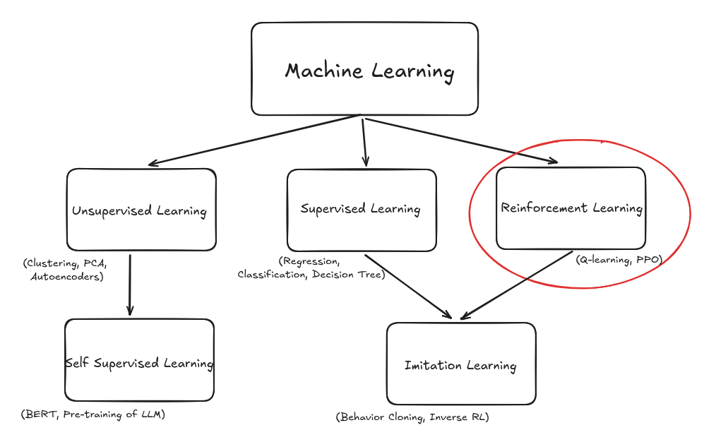
What is reinforcement learning, really?

Reinforcement learning is a type of machine learning. If supervised learning is “here’s the input, here’s the correct label, now learn to produce the correct label”, then reinforcement learning is:

“Here’s the world. Try things. I’ll tell you if you’re doing well or badly.”

Reinforcement learning has two advantages:

• We do not need recorded training data.
• Our model can discover behaviors by itself. As we have seen with our pendulum, it learned a way to swing it up that I could not have demonstrated.

But we do need to explicitly state a reward.

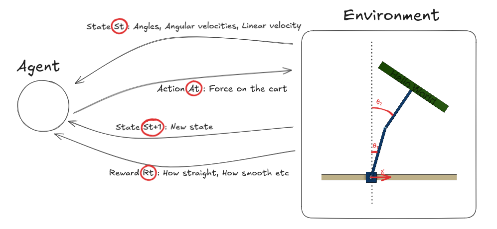
Instead of labeled examples, the agent gets:

• State: what the world looks like right now
• Action: what the agent decides to do
• Reward: a scalar number measuring how good that action (and resulting state) was
• Next state: what the world looks like after the action

This loop repeats over and over.

For the double pendulum:

• State might include:
  • Cart position and velocity
  • First arm angle and angular velocity
  • Second arm angle and angular velocity
• Action:
  • A continuous force to apply to the cart
• Reward:
  • Positive when the arms are upright and the motion is smooth
  • Negative when the arms fall or move too violently (see Part 1 to see our detailed Reward)

The key idea:
The agent is not told what to do. It’s only told how well it did, using the reward signal.

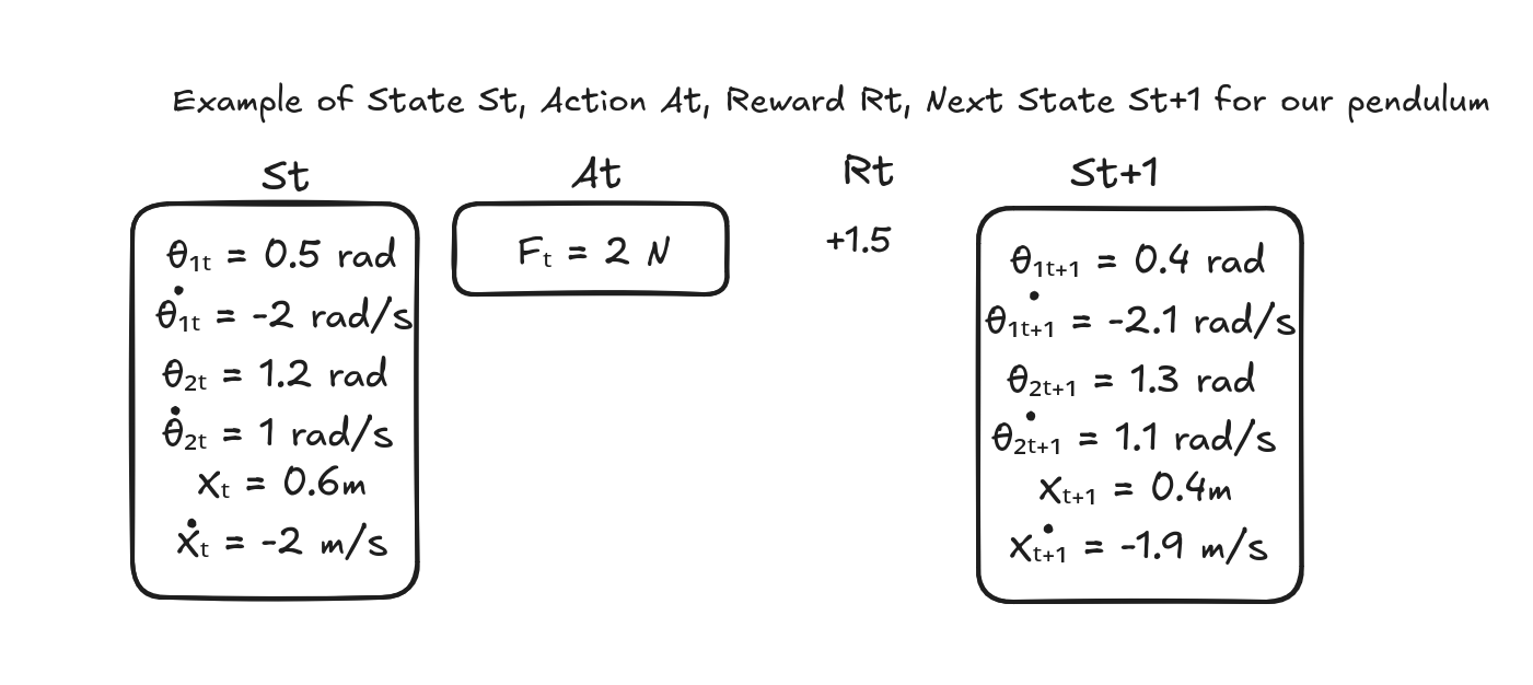
The tuple (state, action, reward, next state) is stored for learning.

After a batch of steps, the agent uses all the accumulated data to update the neural network parameters.

This “collect experience → update network” cycle repeats until the behavior converges to something useful. Over time (and millions of time steps), the agent discovers a strategy (called a policy) that tends to produce high total reward.

Immediate rewards vs. future returns: a crucial distinction

Rewards are computed immediately

At each time step $t$, the environment computes a reward $r_t$ based on:

• The current state $s_t$
• The action $a_t$ that was just taken
• The resulting next state $s_{t+1}$

For our double pendulum, at every control step (every 16.67 ms), the reward function:

• Measures how upright the arms are (position reward)
• Measures how smooth the motion is (velocity penalties)
• Computes a single scalar value: $R_t$

This reward is immediate – it’s computed right after the action is applied, based on what happened in that single time step.

But the agent optimizes for future returns

However, the agent doesn’t just care about the immediate reward. It cares about the total future reward it can expect from this point forward.

This is captured by the return (also called the discounted return):

Where:

• $R_t$ is the immediate reward at time $t$
• $\gamma$ is the discount factor (typically 0.99 or 0.999)
• Future rewards are discounted (weighted less) the further they are in the future

Why discount future rewards?

The discount factor $\gamma$ serves several purposes:

1. Mathematical convenience: Without discounting, infinite-horizon problems can have infinite returns, making optimization impossible.

2. Uncertainty: The further in the future, the less certain we are about what will happen. A reward now is more valuable than the same reward later.

3. Practical behavior: It encourages the agent to achieve rewards sooner rather than later.

For example, with $\gamma = 0.99$:

• A reward of +1.0 at time $t$ contributes +1.0 to the return
• A reward of +1.0 at time $t+1$ contributes +0.99 to the return
• A reward of +1.0 at time $t+10$ contributes only +0.90 to the return

4. Core concepts in RL

Let’s define some core concepts in RL:

4.1 Policy $\pi(a \mid s)$

The policy is the agent’s behavior. Its role is to output an action given a state.

• Input: current state
• Output: probability distribution over actions

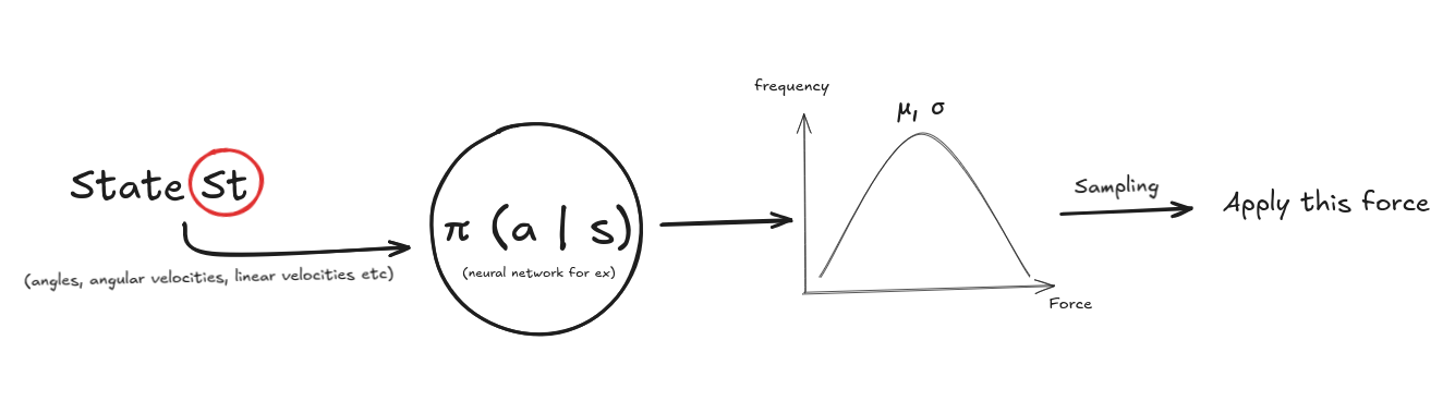
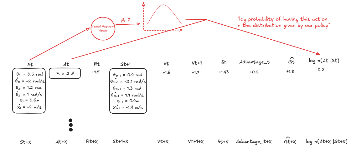
For continuous control like our double pendulum, the policy output is usually a Gaussian distribution:

The policy is usually implemented as a neural network.

• The neural network outputs:
  • A mean vector $\mu(s)$
  • A standard deviation vector $\sigma(s)$ (or sometimes a global $\sigma$)
• The action is sampled as: \(a \sim \mathcal{N}(\mu(s), \sigma(s))\)

This stochasticity is important:
The agent must explore different actions to learn what works, so we allow this by having a statistical distribution of actions rather than a single deterministic action.

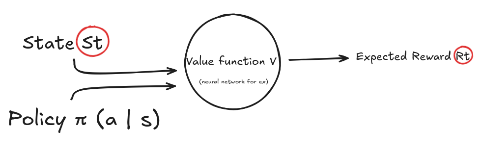
4.2 Value function $V(s)$

The value function tells us:

“Starting from this state, how much total future reward can I expect if I follow my current policy?”

Formally: \(V^\pi(s) = \mathbb{E}\left[\sum_{t=0}^T \gamma^t r_t \mid s_0 = s, \pi\right]\)

“What is my expected total reward given my current state and my current policy”

In practice, we approximate this with another neural network, the critic.

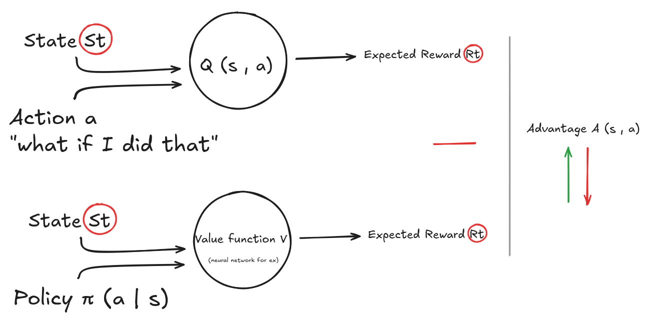
4.3 Advantage function $A(s,a)$

The advantage $A(s,a)$ measures how much better an action turned out to be, compared to following our policy.

One common definition:

Where:

• $Q(s,a)$ is called the action-value function. It is the expected return if we take action $a$ in state $s$ and follow the policy afterwards.

• $V(s)$ is called the state-value function. It is the average expected return if we just follow the policy from state $s$.

• If an action performed better than expected, advantage > 0 → push policy towards that action.
• If it performed worse than expected, advantage < 0 → push policy away from that action.

Intuition with a Simple Example

You’re playing a game:

• In state $s$, following your policy typically gives you 10 points. (This is $V(s) = 10$)
• But taking action $a_1$ gives you 15 points. (This is $Q(s, a_1) = 15$)
• Taking action $a_2$ gives you 9 points. (This is $Q(s, a_2) = 9$)

Then:

• $A(s, a_1) = 15 - 10 = +5$ → better than average
• $A(s, a_2) = 9 - 10 = -1$ → worse than average

Interpretation:

• Your policy should shift probability toward $a_1$ (because it’s better than average)
• And shift probability away from $a_2$ (because it’s worse than average).

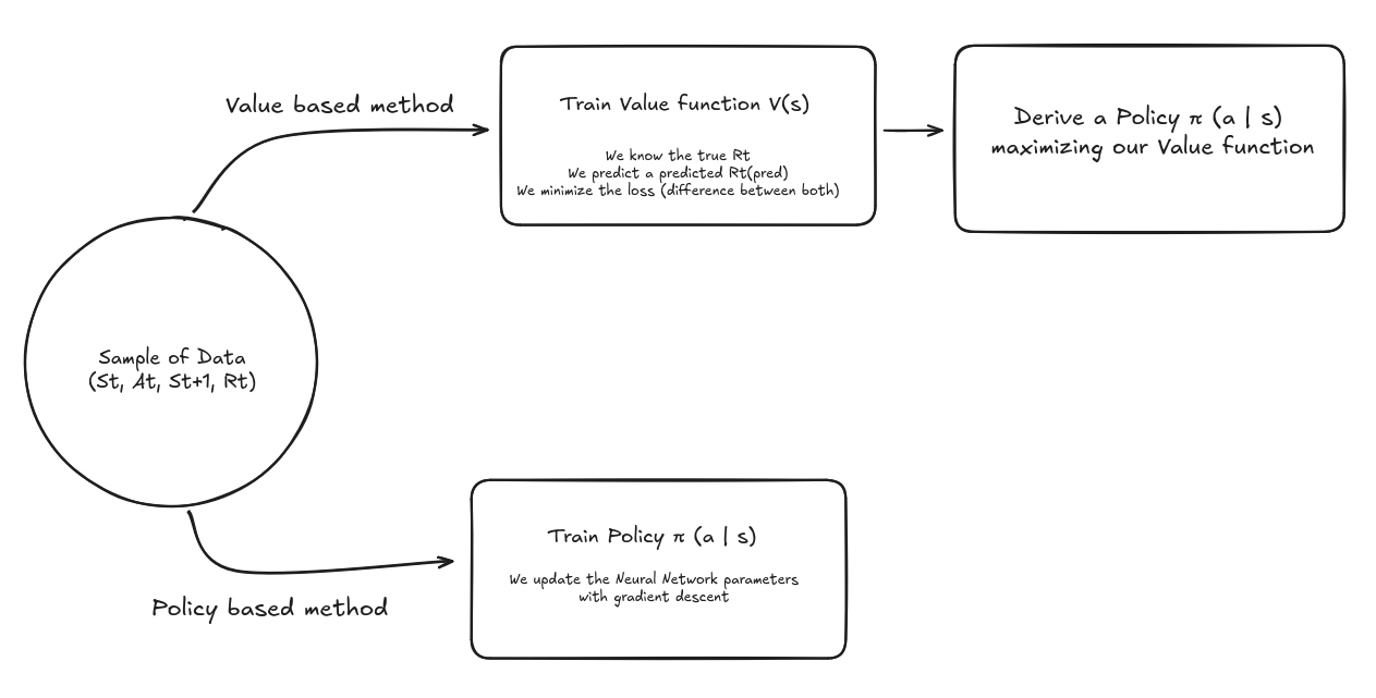
5. Value-based methods vs policy-based methods

There are two broad ways to solve RL problems:

• Value-based methods: learn a value function that maximizes the reward and derive a policy from it (e.g., Q-learning, DQN). Indeed, if I can efficiently predict my future rewards, I can derive a policy that maximizes it.
• Policy-based methods: directly learn a policy that maps states to actions and maximizes the reward.

In the policy-based method, we call $\theta$ the policy parameters of our neural network.
The gradient of the objective with respect to $\theta$ looks like:

Where:

• $\log \pi_\theta(a \mid s)$ is how likely the policy thinks that action is. (we take the log to simplify the gradient maths and provide stability by turning products into sums)
• $G_t$ is our discounted return function seen earlier.

(we took a shortcut to arrive at this formula, if you want the full details, check out here )

Then we can use this gradient to update the policy (neural network) parameters by doing the usual back propagation.
If the reward is high → increase the probability of that action in that state.
If the reward is low → decrease the probability.

Value-based methods are great for small sampled data where the action space is discrete, but they perform weakly in exploration because they tend to directly maximize the reward (greedy).
Policy-based methods are great for continuous action spaces (robotics) and perform better at exploration since stochasticity is built in. They do need more data.

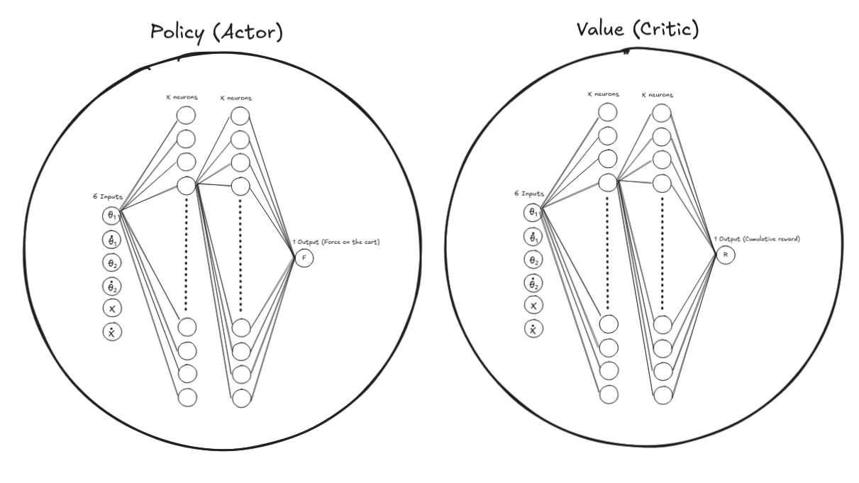
6. The hybrid architecture: actor-critic methods

In policy methods, we need to use $G_t$ in our gradient to update our model parameters. However, $G_t$ is a very noisy signal with high variance: in some episodes an action can lead to a high final reward and in others to a low final reward due to the uncertainty and variability of the future.
Due to this high variance, in order to properly train a policy-based method, we need a lot of episodes and data.
Actor-critic methods solve this high-variance issue by combining both approaches.

In actor-critic methods, we will train both models at the same time:

• A policy that controls our agent and outputs actions
• A value function predicting how good a state is (i.e., the expected future return starting from that state) as we’ve seen earlier.

Instead of using $G_t$ directly, our Actor-Critic method will use the Advantage function we have seen earlier: \(A(s, a) = Q(s, a) - V(s)\)

So the gradient becomes:

Keep in mind that $V(s)$ is a neural network itself now.

Down the rabbit hole: how to compute Q(s, a)?

If the action-value function $Q(s,a)$ is “what is my reward if I perform the action a and follow the policy afterward” and the state-value function $V(s)$ is “what is my reward if I follow the policy”, then we can express everything based on the Critic when we take the difference.
Mathematically:

As we have

Using the value function \(V(s_{t+1})\) of the next state, we can rewrite \(Q(s_t, a_t)\) as:

and so

(it’s an approximation because we use our critic estimate instead of the true value)
($\gamma$ is our discount factor seen before)
It is called the TD-error ($\delta_t$) and we can easily compute it from the $(S_t, A_t, S_{t+1}, R_t)$ data points we collect in each episode and our Critic model $V(s_t)$.

Even deeper: GAE is better than TD-error

TD-error approximates the Advantage function by looking at the difference between the action-value function $Q$ and the state-value function $V$ over one step.
But we can have an even better approximation by looking at the difference over multiple steps.
Instead of just looking at the advantage at time t, we look at the advantages over the rest of the trajectory. We use a parameter $\lambda$ to control how far we look in time.

Recursively we define
\(A_t = \delta_t + (\gamma\lambda)A_{t+1}\) So
\(A_t = \delta_t + (\gamma\lambda)\delta_{t+1} + (\gamma\lambda)^2\delta_{t+2} + ...\)

In practice we can compute $A_t$ at the end of an episode starting from the end and computing it recursively.
$\lambda$ allows us to control how far we want to look:

• $\lambda$ = 0 is equivalent to the TD-error approach, low variance but high bias
• $\lambda$ = 1 is equivalent to the full sample approach similar to the policy method, low bias but high variance.

Full summary of the training loop

To wrap everything up, here is the complete training cycle used in an actor-critic method with GAE. This gives a clear, high-level view of how all the pieces fit together.

1. Initialize the Models

• Initialize both networks (with random weights):
  • Actor: outputs actions given a state.
  • Critic: predicts the value of each state.

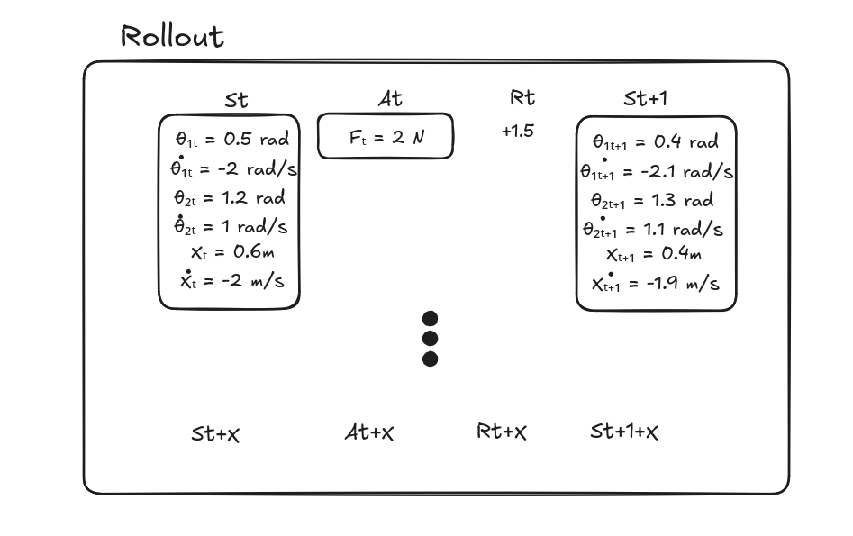
2. Collect a Batch of Experience

• Run the current policy in the environment for a fixed number of steps.
• At each timestep, record:
  • State: $s_t$
  • Action taken: $a_t$
  • Reward received: $r_t$
  • Next state: $s_{t+1}$
• This set of transitions is called a rollout.

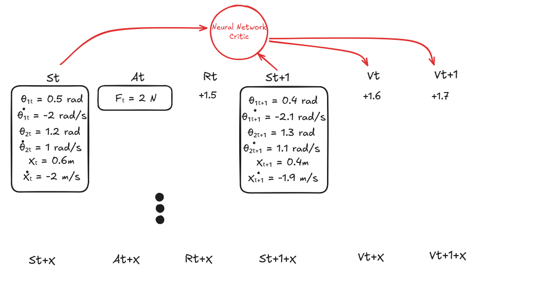
3. Estimate the Values

• Use the critic network to compute value estimates for each state:
  • $V(s_t)$
  • $V(s_{t+1})$

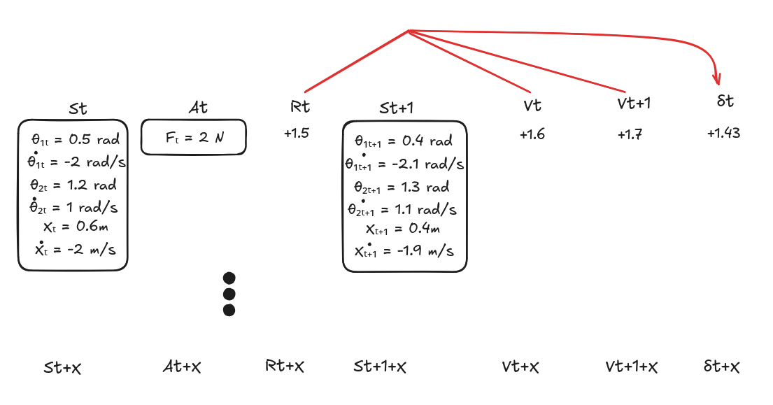
4. Compute the TD-Errors

• For each timestep, compute the temporal-difference error (TD-error): \(\delta_t = R_t + \gamma V(s_{t+1}) - V(s_t)\)
• This measures how “surprising” or “better or worse than expected” each outcome was.

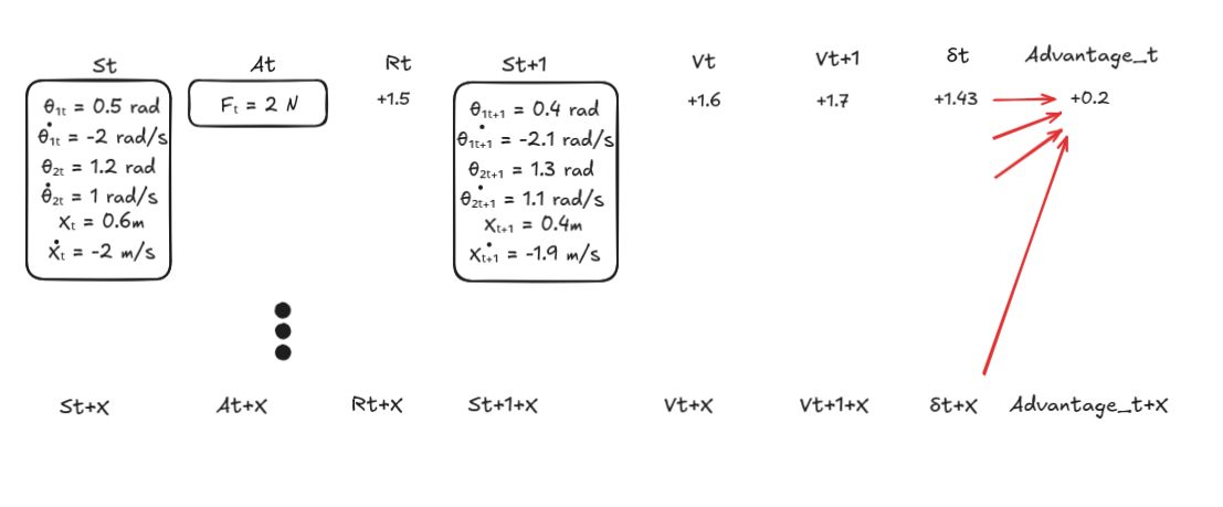
5. Compute the Advantages with GAE

• Compute the advantages using the formula: \(A_t = \delta_t + (\gamma\lambda)\delta_{t+1} + (\gamma\lambda)²\delta_{t+2} + ...\)
• This produces a smoothed, low-variance estimate of the advantage for each action.

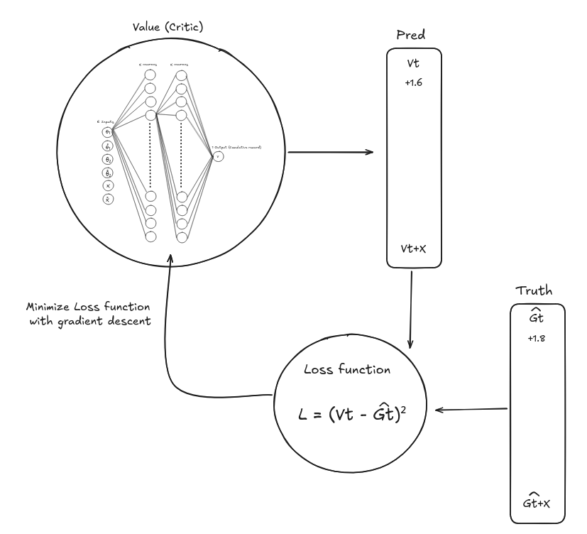
6. Train and Update the Critic

• To train the critic, we compute the return estimate: \(\hat{G}_t = A_t + V(s_t)\)
• This serves as the supervised learning target for the value network.

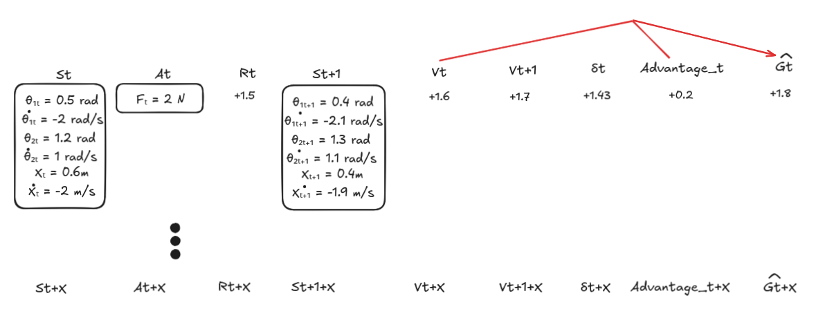
• Update the critic by minimizing the mean-squared error between predicted values and return targets: \(L_{\text{critic}} = (V(s_t) - \hat{G}_t)^2\)

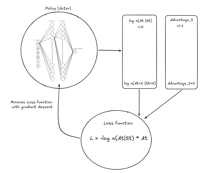
7. Update the Actor

• Using the policy, compute the log probability of each action.

• Update the policy so that actions with positive advantage are more likely, and those with negative advantage are discouraged.
• The basic policy loss is: \(L_{\text{actor}} = -\log \pi(a_t | s_t) \, A_t\)

8. Repeat

• Repeat the loop:
  • Collect new data with the updated policy.
  • Recompute value estimates, TD-errors, advantages, and returns.
  • Update the actor and critic again.
• Over time, both networks improve:
  • The critic predicts values more accurately,
  • The actor learns an increasingly effective policy for the environment.

7. Details behind PPO: Proximal Policy Optimization

Now we get to the algorithm I used to train the double pendulum: PPO (Proximal Policy Optimization).

PPO is popular because it strikes a good balance between:

• Performance: It works very well on complex continuous control tasks.
• Stability: It avoids taking too-large, destabilizing policy updates.
• Simplicity: It’s relatively easy to implement and tune.

7.1 The core idea

Naively, if we use policy gradients, we might make huge updates to the policy after each batch of experience. That can completely break a working policy.

PPO prevents this by constraining how much the policy is allowed to change at each update.

It does this through a clipped objective.

7.2 The probability ratio

PPO compares:

• The old policy $\pi_{\theta_{\text{old}}}$ used to generate data.
• The new policy $\pi_{\theta}$ we’re trying to optimize.

For each state–action pair, we compute the probability ratio (not to be confused with the reward $r_t$):

• If $r_t(\theta) > 1$: the new policy makes that action more likely.
• If $r_t(\theta) < 1$: the new policy makes that action less likely.

We want to increase the likelihood of actions with positive advantage, and decrease for negative advantage. But we don’t want $r_t(\theta)$ to change too much in one update.

7.3 The clipped objective

PPO uses the following (simplified) clipped objective:

Where:

• $\epsilon$ is a small number like 0.1 or 0.2.
• The clip function keeps $r_t(\theta)$ within $[1 - \epsilon, 1 + \epsilon]$.

Intuition:

• For good actions (advantage > 0), we want to increase their probability, but not too much.
• For bad actions (advantage < 0), we want to decrease their probability, but not too much either.

PPO takes the minimum of the unclipped and clipped objective. This effectively penalizes updates that would change the policy too drastically.

The result: conservative, stable learning steps that improve the policy without breaking it.

8. Where did we define all of these in our model?

The policy, value function, and PPO hyperparameters above live in the project config at DoublePendulumIsaacLab/DoublePendulumTraining/source/DoublePendulumTraining/DoublePendulumTraining/tasks/manager_based/doublependulumtraining/agents/skrl_ppo_cfg.yaml.

Specific mappings:

• policy and value: Define the two neural nets (both 128×128 ELU MLPs).
• agent: Sets PPO knobs such as discount_factor ($\gamma$), lambda ($\lambda$), and ratio_clip ($\epsilon$).
• trainer: Controls rollouts (batch collection length) and timesteps (total training duration).

Our config for training the model in Isaac Lab is defined in ‘skrl_ppo_cfg.yaml’

Here is the full config:

seed: 42


# Models are instantiated using skrl's model instantiator utility
# https://skrl.readthedocs.io/en/latest/api/utils/model_instantiators.html
models:
  separate: False
  policy:  # see gaussian_model parameters
    class: GaussianMixin
    clip_actions: False
    clip_log_std: True
    min_log_std: -20.0
    max_log_std: 2.0
    initial_log_std: 0.0
    network:
      - name: net
        input: OBSERVATIONS
        # Increased network size from [32, 32] to [128, 128] for better learning capacity
        # Balancing a double pendulum requires more complex control, so a larger network
        # can learn more sophisticated balancing strategies
        # 128 units per layer provides sufficient capacity for this challenging task
        layers: [128, 128]
        activations: elu
    output: ACTIONS
  value:  # see deterministic_model parameters
    class: DeterministicMixin
    clip_actions: False
    network:
      - name: net
        input: OBSERVATIONS
        # Increased network size from [32, 32] to [128, 128] for better value estimation
        # A larger value network can better predict expected returns for complex balancing
        # Matching policy network size for consistency
        layers: [128, 128]
        activations: elu
    output: ONE


# Rollout memory
# https://skrl.readthedocs.io/en/latest/api/memories/random.html
memory:
  class: RandomMemory
  memory_size: -1  # automatically determined (same as agent:rollouts)


# PPO agent configuration (field names are from PPO_DEFAULT_CONFIG)
# https://skrl.readthedocs.io/en/latest/api/agents/ppo.html
agent:
  class: PPO
  rollouts: 32
  learning_epochs: 8
  mini_batches: 8
  discount_factor: 0.99
  lambda: 0.95
  # Learning rate: Slightly reduced for more stable learning with larger network
  # The larger network (128x128) benefits from a slightly lower learning rate
  learning_rate: 3.0e-04
  learning_rate_scheduler: KLAdaptiveLR
  learning_rate_scheduler_kwargs:
    kl_threshold: 0.008
  state_preprocessor: RunningStandardScaler
  state_preprocessor_kwargs: null
  value_preprocessor: RunningStandardScaler
  value_preprocessor_kwargs: null
  random_timesteps: 0
  learning_starts: 0
  grad_norm_clip: 1.0
  ratio_clip: 0.2
  value_clip: 0.2
  clip_predicted_values: True
  entropy_loss_scale: 0.0
  value_loss_scale: 2.0
  kl_threshold: 0.0
  rewards_shaper_scale: 0.1
  time_limit_bootstrap: False
  # logging and checkpoint
  experiment:
    directory: "doublependulumtraining"
    experiment_name: ""
    # write_interval: Number of timesteps between TensorBoard log writes
    # Set to 1 to log every step, or a higher number to log less frequently
    # For training analysis, logging every 10-100 steps is usually sufficient
    write_interval: 10  # Log to TensorBoard every 10 timesteps
    # checkpoint_interval: Number of timesteps between model checkpoints
    # Set to a higher number to save less frequently (saves disk space)
    checkpoint_interval: 100  # Save checkpoint every 100 timesteps


# Sequential trainer
# https://skrl.readthedocs.io/en/latest/api/trainers/sequential.html
trainer:
  class: SequentialTrainer
  # timesteps: Total number of timesteps to train
  # 30000 timesteps = 30000 / (rollouts=32) ≈ 937 iterations
  # Each iteration processes 32 rollouts (32 episodes worth of data)
  # Chosen to give enough updates while keeping wall-clock time reasonable
  timesteps: 30000
  environment_info: log

We define two neural networks, policy and value, corresponding to the policy and value functions discussed earlier. Both are 128×128 ELU MLPs.
The PPO setup uses rollouts: 32, meaning each iteration gathers 32 steps before running updates. learning_epochs: 8 means we reuse that batch eight times per iteration.
Key PPO parameters (discount_factor, lambda, ratio_clip, value_clip) map directly to the concepts above. learning_rate and the KL-based scheduler control step size, and entropy_loss_scale would encourage exploration (kept at 0 here).
—

Other topics in RL

Domain randomization for sim-to-real

• Randomize physics and visuals during simulation (masses, friction, motor gains, sensor noise, textures, lights) so the policy trains on a distribution, not a single “perfect” simulator.
• The goal is a policy that’s robust to reality’s quirks because it has already seen many variations.
• Works well with Isaac Lab: easy to sample parameters each episode, log what was used, and replay troublesome seeds when you see real-world failures.

Two areas I’ll cover in future articles because they pair nicely with continuous control:

Imitation learning (behavior cloning / DAGGER)

• Train a policy directly from demonstrations instead of (or before) reward-based RL.
• Useful when you can teleoperate the robot or script a decent controller to create expert trajectories.
• Often combined with PPO: pretrain with imitation to get a stable starting policy, then fine-tune with RL for robustness.

VLA (Vision–Language–Action) policies

• Combine perception (images), language instructions, and action generation in one model.
• Great for tasks where you want to say “place the upper link over the marker” rather than craft a reward for every nuance.
• Still data-hungry; simulators like Isaac Lab help generate diverse visual data before real-world transfer.