<?xml version="1.0" encoding="utf-8"?><feed xmlns="http://www.w3.org/2005/Atom" ><generator uri="https://jekyllrb.com/" version="3.10.0">Jekyll</generator><link href="https://nrdrgz.github.io/feed.xml" rel="self" type="application/atom+xml" /><link href="https://nrdrgz.github.io/" rel="alternate" type="text/html" /><updated>2026-10-28T09:00:06+00:00</updated><id>https://nrdrgz.github.io/feed.xml</id><title type="html">Welcome to Nico’s blog</title><subtitle>Hope you&apos;ll learn something new!</subtitle><author><name>Nicolas Rodriguez</name></author><entry><title type="html">Monkey see, monkey do: teaching robots by demonstration with Imitation Learning</title><link href="https://nrdrgz.github.io/2026/10/28/imitation-learning-act-pi05-vla/" rel="alternate" type="text/html" title="Monkey see, monkey do: teaching robots by demonstration with Imitation Learning" /><published>2026-10-28T00:00:00+00:00</published><updated>2026-10-28T00:00:00+00:00</updated><id>https://nrdrgz.github.io/2026/10/28/imitation-learning-act-pi05-vla</id><content type="html" xml:base="https://nrdrgz.github.io/2026/10/28/imitation-learning-act-pi05-vla/"><![CDATA[<p>It’s been a while since my last post. I was busy teaching robots to do stuff, so let’s wrap our minds around it.</p>

<video class="img-large" autoplay="" loop="" muted="" playsinline="">
  <source src="/assets/images/posts/imitation-learning/box_opening.mp4" type="video/mp4" />
</video>

<div class="story-bar">
That's my Seeed Studio robotic arm opening the door of an electrical cabinet. It never learnt in simulation. I just grabbed the arm, showed it how to do the task a few dozen times, hit train, and let it figure out the rest. <br />
<br />
After spending some time on the reinforcement learning side with my <a class="link-prominent" href="https://nrdrgz.github.io/2025/11/06/double-pendulum-isaaclab/" target="_blank" rel="noopener">inverted double pendulum</a>
, this feels almost like cheating.
</div>

<p>In my <a class="link-prominent" href="https://nrdrgz.github.io/2025/12/02/double-pendulum-rl-deep-dive/" target="_blank" rel="noopener">last article</a>
, we taught a robot to balance a pendulum using reinforcement learning. We never told it <em>what</em> to do. We only told it <em>how well</em> it did, through a reward signal, and let it discover a strategy on its own across millions of simulation steps.</p>

<p>This time, we’re doing the exact opposite. We’re going to <em>show</em> the robot what to do.</p>

<p>Welcome to <strong>imitation learning</strong>.</p>

<h2 id="from-rewards-to-demonstrations">From rewards to demonstrations</h2>

<p>Let’s put them next to each other before going further.</p>

<p>With <strong>reinforcement learning</strong>, you don’t need any data. But there’s a catch (actually a few):</p>
<ul>
  <li>You have to hand-craft a reward function. (Remember how much time we spent tweaking those reward weights for the pendulum?)</li>
  <li>You usually need a simulator, because the agent learns by trial and error, and you can’t crash a real robot a million times.</li>
  <li>And then you let it explore for millions of steps until it stumbles onto something good.</li>
</ul>

<p>With <strong>imitation learning</strong>, you flip the whole thing around. The robot learns by copying <em>you</em>. The price you pay is that now you need real-life demonstrations.</p>

<div class="callout">
Reinforcement learning: "Here's the world. Try things. I'll tell you if you're doing well or badly." <br />
Imitation learning: "Here's how I did it. Now you do it."
</div>

<p>That sounds much simpler, and in many ways it is. It’s a big part of why robot manipulation has exploded recently. But imitation learning has its own dirty little secret, one that bit me hard at a hackathon last December. Hold that thought, we’ll get to it.</p>

<h2 id="what-is-imitation-learning-really">What is imitation learning, really?</h2>

<p>At its core, the simplest form of imitation learning is just <strong>supervised learning</strong> wearing a robotics costume.</p>

<p>Think back to how we framed things last time. Supervised learning is “here’s the input, here’s the correct label, now learn to produce the label.” Imitation learning, in its most basic form (called <strong>behavior cloning</strong>), is exactly that:</p>

<ul>
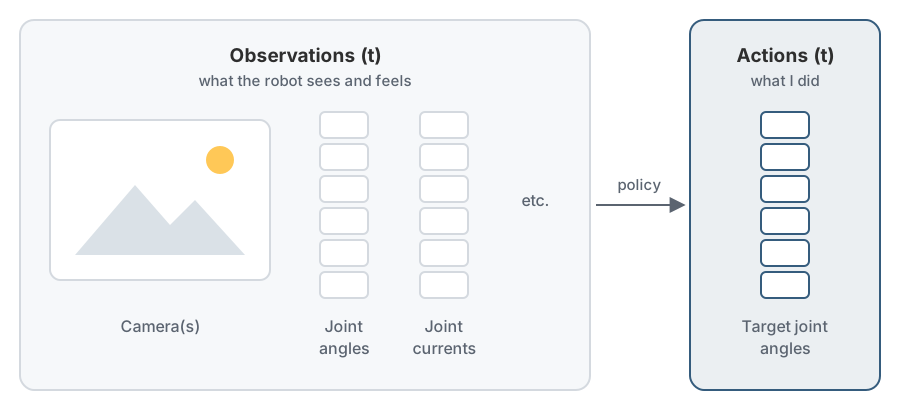
  <li><strong>Input</strong>: what the robot sees and feels right now. The camera image(s) and the position of each joint, sometimes more, like motor currents or force sensors.</li>
  <li><strong>Label</strong>: the action I took at that exact moment. Where I moved each joint.</li>
</ul>

<p>You record a bunch of <code class="language-plaintext highlighter-rouge">(observation, action)</code> pairs while doing the task, and you train a neural network to map one to the other. That’s it. The robot is literally cloning your behavior, one moment at a time.</p>

<p><img src="/assets/images/posts/imitation-learning/observation_actions.svg" alt="Behavior cloning as supervised learning" class="img-large" /></p>

<p>There are fancier flavors of imitation learning out there (things like DAgger, or inverse reinforcement learning where you try to <em>recover</em> the reward function from demonstrations). But the models everyone is excited about right now, including the two we’ll dig into, are built on good old behavior cloning. So that’s what we’ll focus on.</p>

<p>The interesting part isn’t the idea, which is almost embarrassingly simple. It’s everything that goes wrong when you actually try it, and the clever tricks people invented to fix it.</p>

<h2 id="collecting-demonstrations-teleoperation">Collecting demonstrations: teleoperation</h2>

<p>Before any of that, you need data. And in robotics, the data <em>is</em> the model. There’s no giant dataset of “opening electrical cabinets” sitting on the internet. You have to make it yourself.</p>

<p>The way you do this is <strong>teleoperation</strong>. You physically move the robot through the task while recording everything.</p>

<p>The classic setup is a <strong>leader and a follower</strong>. You have two arms: a leader arm that you move by hand, and a follower arm that mirrors its movements. As you guide the leader through the task, the follower copies it, and the whole time you’re recording the joint positions and the camera feed. Each successful run is one “episode.”</p>

<p>I used two different arms across my experiments:</p>
<ul>
  <li>The <strong>SO-101</strong>, which I’d worked with before, has <strong>5 degrees of freedom</strong>.</li>
  <li>The <strong>Seeed Studio arm</strong> has <strong>6 degrees of freedom</strong>.</li>
</ul>

<p>That extra degree of freedom matters more than it sounds. With 5 DoF, there are orientations the gripper simply can’t reach. The 6th joint gives you a free wrist, which for a task like reaching in at an angle to grab a cabinet door is the difference between “possible” and “constantly fighting the robot.” The flip side: every degree of freedom you add is one more thing the model has to learn to coordinate.</p>

<p>This is me teleoperating a Seeed Studio follower arm with a leader arm:</p>

<video class="img-large" autoplay="" loop="" muted="" playsinline="">
  <source src="/assets/images/posts/imitation-learning/teleoperation.mp4" type="video/mp4" />
</video>

<p>Data collection is repetitive and a little tedious. You do the same task over and over, a few dozen times, trying to be consistent but also varied enough that the model doesn’t memorize one exact trajectory. You quickly develop a deep respect for anyone who collects thousands of episodes.</p>

<p>And here’s where I learned my lesson the hard way.</p>

<div class="story-bar">
Last December, I was at a hackathon with a team. We spent the whole first day collecting demonstrations and training a model to do a manipulation task. By the end of the day it worked beautifully. We were thrilled. <br />
<br />
We came back the next morning, ran the exact same model... and it was a disaster. The robot fumbled, missed, did nonsense. Nothing about the code or the model had changed overnight. <br />
<br />
After a confused hour of debugging, we figured it out. One of my teammates, who had been sitting in the background of the camera frame during all of yesterday's recordings, had simply sat down in a different spot. The model had quietly learned that "my teammate is sitting *there*" was part of what the task looked like. Move him, and the whole thing fell apart. <br />
<br />
We still managed to give the judges a very nice demo, by having my teammate sit back exactly where he had been sitting during teleoperation.
</div>

<p>We laughed about it at the time. But that story is actually the perfect doorway into the single most important concept in imitation learning, and the thing every model in this space is fighting against. Let me first show you the model I used, and then come back to <em>why</em> my teammate broke it.</p>

<h2 id="under-the-hood-the-act-model">Under the hood: the ACT model</h2>

<p>The model I trained from scratch for these tasks is called <strong>ACT</strong>, which stands for <strong>Action Chunking with Transformers</strong>. It came out of the <a class="link-prominent" href="https://tonyzhaozh.github.io/aloha/" target="_blank" rel="noopener">ALOHA project</a>
 and is one of the most popular starting points for robot imitation learning today.</p>

<p>Let’s build it up piece by piece, because every part of it is a fix for a specific problem.</p>

<h3 id="the-problem-predicting-one-action-at-a-time-is-fragile">The problem: predicting one action at a time is fragile</h3>

<p>The naive behavior cloning we described earlier predicts a single action from a single observation. Then the robot moves, observes again, predicts the next action, and so on.</p>

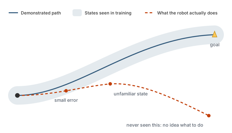
<p>The problem is that tiny errors <strong>compound</strong>. The robot makes a small mistake, which puts it in a slightly unfamiliar state, where it makes a slightly bigger mistake, which puts it somewhere even more unfamiliar… and within a second or two it has drifted somewhere it has never seen and has no idea what to do. (We’ll formalize this in the next section, it has a name.)</p>

<h3 id="the-fix-action-chunking">The fix: action chunking</h3>

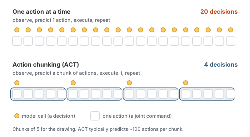
<p>Instead of predicting one action, ACT predicts a whole <strong>chunk</strong> of future actions at once, say the next ~100 steps.</p>

<p><img src="/assets/images/posts/imitation-learning/action_chunking.svg" alt="Action chunking" class="img-large" /></p>

<p>Why does this help? Because it shortens the number of decisions the model has to make. If you commit to 100 actions at a time, you’ve effectively divided the length of your task by 100, and there are far fewer opportunities for errors to accumulate and snowball. The robot follows a short, coherent plan instead of nervously re-deciding everything at every single step.</p>

<h3 id="smoothing-it-out-temporal-ensembling">Smoothing it out: temporal ensembling</h3>

<p>There’s a subtlety. If you predict a chunk, execute all of it, then predict the next chunk, you get a little “jerk” at the boundary between chunks where the new plan disagrees with the old one.</p>

<p>ACT’s trick is <strong>temporal ensembling</strong>. It actually queries the model at <em>every</em> timestep, producing overlapping chunks, and then averages the predictions for the current moment across all the chunks that have an opinion about it. The result is smooth, continuous motion instead of jerky stop-and-go. (Notice the philosophy is the opposite of my pendulum, where I <em>penalized</em> jerky motion in the reward. Here there’s no reward to do that, so the smoothing is baked into the architecture.)</p>

<h3 id="the-clever-bit-the-cvae-and-human-messiness">The clever bit: the CVAE and human messiness</h3>

<p>Here’s the part I find most elegant.</p>

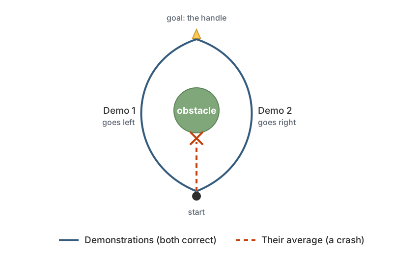
<p>When a human demonstrates a task multiple times, the demonstrations are <strong>multimodal</strong>. You don’t do the exact same thing every time. Sometimes you approach the cabinet handle from slightly above, sometimes from the side. Both are correct.</p>

<p>A naive network trained to minimize error on this data does something terrible: it averages the two valid approaches and aims for the middle, which might be straight into an obstacle. Averaging two correct answers can give you a very wrong one.</p>

<p><img src="/assets/images/posts/imitation-learning/multimodal_averaging.svg" alt="Averaging two valid demonstrations" class="img-large" /></p>

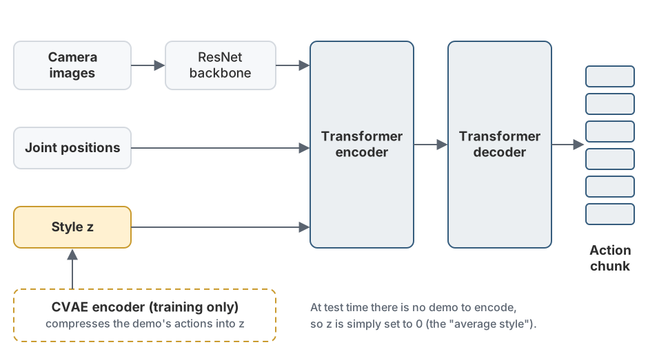
<p>ACT solves this by being a <strong>CVAE</strong> (Conditional Variational Autoencoder). The intuition, without drowning in the math:</p>

<ul>
  <li>During training, an encoder looks at the demonstration and compresses its “style” into a small latent variable $z$. Think of $z$ as capturing <em>which way</em> you happened to do it this time.</li>
  <li>The main network (a transformer encoder-decoder) then generates the action chunk conditioned on the images, the joint positions, <strong>and</strong> this style variable $z$.</li>
  <li>The model is trained with two objectives: an $L_1$ loss that says “reproduce the demonstrated actions,” and a KL-divergence term that keeps the space of styles $z$ well-behaved (close to a simple Gaussian).</li>
</ul>

\[L = \underbrace{\| a - \hat{a} \|_1}_{\text{reproduce the actions}} + \beta \underbrace{D_{\text{KL}}\big(q(z \mid a, s) \,\|\, \mathcal{N}(0, I)\big)}_{\text{keep the style space tidy}}\]

<p>At test time, you simply set $z = 0$ (the “average style”) and let the network produce a coherent action chunk. Because the multimodality was absorbed into $z$ during training, the network no longer has to average incompatible behaviors. It picks one clean way to do the task instead of mushing them together.</p>

<p><img src="/assets/images/posts/imitation-learning/act_architecture.svg" alt="ACT architecture" class="img-large" /></p>

<p>Put it all together: ResNet backbones turn the camera images into features, a transformer fuses those with the joint positions and the latent $z$, and out comes a chunk of smooth, human-like actions. Trained on a few dozen of my teleoperated episodes, this is what learned to open the cabinet.</p>

<h2 id="the-achilles-heel-distribution-shift">The Achilles heel: distribution shift</h2>

<p>Now let’s come back to my hackathon teammate.</p>

<p>The fundamental weakness of behavior cloning has a name: <strong>distribution shift</strong> (or covariate shift). It’s the formal version of the compounding-errors problem we hand-waved at earlier.</p>

<p>Here’s the issue. The model only ever saw the states that appear in your demonstrations. As long as it stays on that familiar path, it knows what to do. But the moment it drifts even slightly off-distribution, into a state it never saw in training, it’s flying blind. And because each mistake pushes it further from familiar territory, errors don’t just add up, they <strong>compound</strong>.</p>

<p><img src="/assets/images/posts/imitation-learning/distribution_shift.svg" alt="Distribution shift" class="img-large" /></p>

<p>Action chunking helps a lot here, because committing to a short plan gives errors fewer chances to snowball. But it doesn’t <em>cure</em> the problem. Nothing fully does, short of collecting more and better data.</p>

<p>And this is exactly what happened at the hackathon. The model didn’t actually learn “open the cabinet.” It learned to reproduce the pixels it saw during training, and my teammate sitting in the background was one of those pixels. When he moved, the input no longer matched anything in the training distribution, and the robot was instantly off-distribution, flying blind. It hadn’t learned the <em>task</em>. It had learned the <em>data</em>.</p>

<div class="callout">
This is the fundamental bargain of imitation learning. It's wonderfully easy to train, because it's just supervised learning. But your model is only ever as good, and as general, as the demonstrations you give it. It imitates everything in your data, including the things you didn't mean to teach it.
</div>

<p>So how do we get past this? How do we get robots that actually understand the task, that generalize to a cabinet they’ve never seen, in a kitchen they’ve never been in, with a teammate sitting wherever he likes? That’s the frontier, and it’s where things get really exciting.</p>

<h2 id="scaling-up-from-one-task-to-generalist-robots">Scaling up: from one task to generalist robots</h2>

<p>The ACT model I trained does exactly one thing: open one cabinet. Train it on a new task and you start more or less from scratch. That doesn’t scale. You can’t collect demonstrations for every task a robot might ever face.</p>

<p>The big idea on the frontier is the same one that transformed language and vision: <strong>scale</strong>. Instead of one small model per task, train one enormous model on a huge, diverse pile of robot data, across many tasks, many robots, and many environments. With enough variety, the model stops memorizing specific trajectories and starts learning something closer to general manipulation skills.</p>

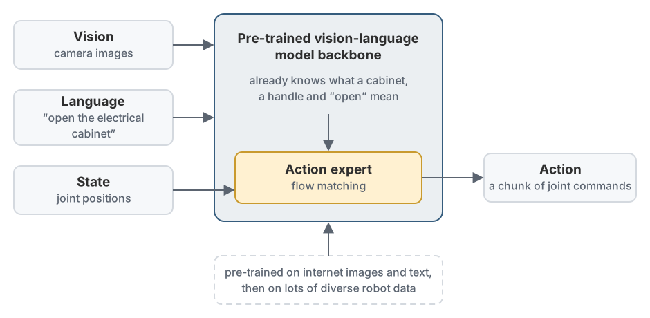
<p>These models are called <strong>VLAs</strong>: <strong>Vision-Language-Action</strong> models.</p>

<p><img src="/assets/images/posts/imitation-learning/vla.svg" alt="Vision Language Action model" class="img-large" /></p>

<p>The name says it all. A VLA fuses three things into a single model:</p>
<ul>
  <li><strong>Vision</strong>: what the robot sees through its cameras.</li>
  <li><strong>Language</strong>: an instruction in plain English, like <em>“open the electrical cabinet.”</em></li>
  <li><strong>Action</strong>: the joint commands sent to the robot.</li>
</ul>

<p>The “language” part is the game-changer. These models are typically built on top of a pre-trained <strong>vision-language model</strong> (the same kind of model that can look at a photo and describe it). That backbone already knows a staggering amount about the world from internet-scale data: what a cabinet is, what a handle is, what “open” means. The robot doesn’t have to learn all of that from your forty demonstrations. It just has to connect that existing knowledge to motor actions.</p>

<h3 id="fine-tuning-pi05">Fine-tuning Pi0.5</h3>

<p>The VLA I got my hands on is <strong>Pi0.5</strong> (π0.5), from <a class="link-prominent" href="https://www.physicalintelligence.company/blog/pi05" target="_blank" rel="noopener">Physical Intelligence</a>
. It’s one of the most capable open generalist robot policies available, explicitly designed for <strong>open-world generalization</strong>, the ability to operate in homes and environments it has never seen.</p>

<p>The contrast with ACT is striking:</p>
<ul>
  <li>Training <strong>ACT</strong> from scratch, the model knows nothing. Your few dozen episodes have to teach it the entire task from zero.</li>
  <li>Fine-tuning <strong>Pi0.5</strong>, the model already understands cabinets, doors, handles, and the general physics of manipulation. Your episodes just nudge a knowledgeable generalist toward your specific setup. You need far less data to get something that generalizes far better.</li>
</ul>

<p>One more technical nugget worth knowing, because it’s a genuinely different approach from ACT’s CVAE. To generate its continuous actions, Pi0.5 uses an <strong>action expert</strong> trained with <strong>flow matching</strong>.</p>

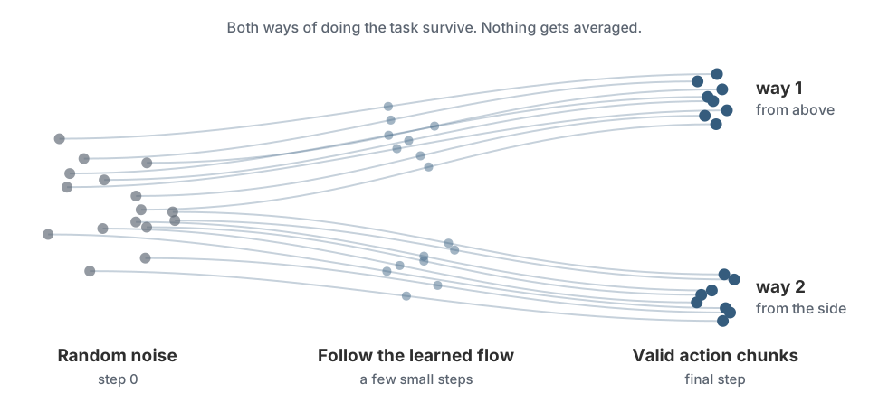
<p>You can think of flow matching as a cousin of the diffusion models behind AI image generators. Instead of producing an action in one shot, the model starts from pure random noise and learns a “velocity field” that smoothly <em>flows</em> that noise, over a few steps, into a real action chunk. The beautiful thing is that this handles the multimodality problem we discussed earlier very naturally: just like an image generator can produce many different valid images, flow matching can produce many different valid ways to do the task, without averaging them into mush. It’s solving the same problem ACT’s latent $z$ solves, but with a much more powerful and scalable tool.</p>

<p><img src="/assets/images/posts/imitation-learning/flow_matching.svg" alt="Flow matching intuition" class="img-large" /></p>

<h2 id="imitation-learning-vs-reinforcement-learning">Imitation learning vs. reinforcement learning</h2>

<p>Now that we’ve been through both this article and the <a class="link-prominent" href="https://nrdrgz.github.io/2025/12/02/double-pendulum-rl-deep-dive/" target="_blank" rel="noopener">RL deep dive</a>
, we can put them side by side honestly.</p>

<table>
  <thead>
    <tr>
      <th> </th>
      <th>Reinforcement Learning</th>
      <th>Imitation Learning</th>
    </tr>
  </thead>
  <tbody>
    <tr>
      <td><strong>What you provide</strong></td>
      <td>A reward function</td>
      <td>Demonstrations</td>
    </tr>
    <tr>
      <td><strong>Needs a simulator?</strong></td>
      <td>Usually yes</td>
      <td>No, you can train on real data</td>
    </tr>
    <tr>
      <td><strong>How it learns</strong></td>
      <td>Trial and error, exploration</td>
      <td>Copying examples</td>
    </tr>
    <tr>
      <td><strong>Can discover new behavior?</strong></td>
      <td>Yes (remember the pendulum swing-up I couldn’t have demonstrated)</td>
      <td>No, it only imitates what it’s shown</td>
    </tr>
    <tr>
      <td><strong>Main weakness</strong></td>
      <td>Reward design and sim-to-real gap</td>
      <td>Distribution shift, only as good as your data</td>
    </tr>
    <tr>
      <td><strong>Great for</strong></td>
      <td>Dynamic, hard-to-demonstrate skills (locomotion, balancing)</td>
      <td>Manipulation, anything a human can easily demonstrate</td>
    </tr>
  </tbody>
</table>

<p>Neither one is “better.” They’re tools for different jobs. RL shines when the behavior is hard to demonstrate but easy to score (how would you teleoperate a robot into balancing my chaotic double pendulum?). Imitation shines when the behavior is easy to demonstrate but hard to score (what’s the reward function for “open a cabinet nicely”?).</p>

<div class="callout">
The most exciting part is that the future probably isn't one or the other, it's <strong>both</strong>. You can use imitation learning to bootstrap a sensible starting policy from demonstrations, then use reinforcement learning to refine it and make it robust, going beyond what a human ever showed it. Imitation gets you to "competent" fast and RL pushes you to "superhuman."
</div>

<h2 id="whats-next-toward-robots-that-imagine">What’s next: toward robots that imagine</h2>

<p>So we’ve now seen two of the big paradigms in modern robot learning. We <em>tell</em> a robot what good looks like with rewards, or we <em>show</em> it what to do with demonstrations. Both have a frustrating limitation in common, though: they need an enormous amount of experience, either millions of simulation steps or piles of demonstrations, because the robot has no real <em>model</em> of how the world works. It can’t think ahead.</p>

<p>What if a robot could build its own internal simulator of reality, watch a situation, and <em>imagine</em> what would happen if it tried something, all in its head, before moving a single motor?</p>

<p>That’s the idea behind <strong>world models</strong>, and it might be the thing that ties this whole series together: from rewards, to demonstrations, to imagination. We’ll write an article about these.</p>

<div class="callout">
Imitation learning is one of the most accessible ways to get into modern robotics. You don't need a reward function or a simulator, just an arm, a camera, and the patience to show it what to do a few dozen times. With tools like <a class="link-prominent" href="https://github.com/huggingface/lerobot" target="_blank" rel="noopener">LeRobot</a>
 and affordable arms like the SO-101 and the Seeed Studio arm, there's never been a better time to teach a robot something yourself. Just keep an eye on who's sitting in the background.
</div>]]></content><author><name>Nicolas Rodriguez</name></author><summary type="html"><![CDATA[No reward functions, no simulator. Just show the robot what to do. A practical and intuitive tour of imitation learning, the ACT model, and the road to VLAs like Pi0.5.]]></summary></entry><entry><title type="html">(Part 2) Behind the scenes: how reinforcement learning and PPO actually work</title><link href="https://nrdrgz.github.io/2025/12/02/double-pendulum-rl-deep-dive/" rel="alternate" type="text/html" title="(Part 2) Behind the scenes: how reinforcement learning and PPO actually work" /><published>2025-12-02T00:00:00+00:00</published><updated>2025-12-02T00:00:00+00:00</updated><id>https://nrdrgz.github.io/2025/12/02/double-pendulum-rl-deep-dive</id><content type="html" xml:base="https://nrdrgz.github.io/2025/12/02/double-pendulum-rl-deep-dive/"><![CDATA[<p>In <a class="link-prominent" href="https://nrdrgz.github.io/2025/11/06/double-pendulum-isaaclab/" target="_blank" rel="noopener">Part 1</a>
, we built and trained an inverted double pendulum in Isaac Lab.<br />
We focused on the practical side: building the URDF, setting up the environment, defining rewards, and running PPO in simulation.</p>

<p>In this article, I want to open the black box.</p>

<p>We’ll walk through:</p>

<ul>
  <li>What <strong>reinforcement learning (RL)</strong> really is (in practical terms)</li>
  <li>How to think about the <strong>agent</strong>, <strong>environment</strong>, <strong>states</strong>, <strong>actions</strong>, and <strong>rewards</strong></li>
  <li>What <strong>policy gradients</strong> are and why they’re a good fit for continuous control</li>
  <li>How <strong>PPO (Proximal Policy Optimization)</strong> works under the hood</li>
  <li>How all of this applies to our <strong>double pendulum</strong> example</li>
</ul>

<div class="story-bar">
I can only encourage you to take a look at the fantastic <a class="link-prominent" href="https://huggingface.co/learn/deep-rl-course/en/unit0/introduction" target="_blank" rel="noopener">Hugging Face Deep Reinforcement Learning course</a>
, from which I learned a lot before experimenting with Isaac Lab and writing this article.
</div>

<h2 id="what-is-reinforcement-learning-really">What is reinforcement learning, really?</h2>

<p>Reinforcement learning is a type of machine learning.
If supervised learning is “<strong>here’s the input, here’s the correct label, now learn to produce the correct label</strong>”, then reinforcement learning is:</p>

<blockquote>
  <p><strong>“Here’s the world. Try things. I’ll tell you if you’re doing well or badly.”</strong></p>
</blockquote>

<p><img src="/assets/images/posts/double-pendulum-deep-dive/hierarchy.png" alt="Hierarchy" class="img-large" /></p>

<p>Reinforcement learning has two advantages:</p>
<ul>
  <li>We do not need recorded training data.</li>
  <li>Our model can discover behaviors by itself. As we have seen with our pendulum, it learned a way to swing it up that I could not have demonstrated.</li>
</ul>

<p>But we do need to explicitly state a reward.</p>

<p>Instead of labeled examples, the agent gets:</p>

<ul>
  <li><strong>State</strong>: what the world looks like right now</li>
  <li><strong>Action</strong>: what the agent decides to do</li>
  <li><strong>Reward</strong>: a scalar number measuring how good that action (and resulting state) was</li>
  <li><strong>Next state</strong>: what the world looks like after the action</li>
</ul>

<p>This loop repeats over and over.</p>

<p>For the <strong>double pendulum</strong>:</p>

<ul>
  <li><strong>State</strong> might include:
    <ul>
      <li>Cart position and velocity</li>
      <li>First arm angle and angular velocity</li>
      <li>Second arm angle and angular velocity</li>
    </ul>
  </li>
  <li><strong>Action</strong>:
    <ul>
      <li>A <strong>continuous force</strong> to apply to the cart</li>
    </ul>
  </li>
  <li><strong>Reward</strong>:
    <ul>
      <li>Positive when the arms are upright and the motion is smooth</li>
      <li>Negative when the arms fall or move too violently
(see Part 1 to see our detailed Reward)</li>
    </ul>
  </li>
</ul>

<p><img src="/assets/images/posts/double-pendulum-deep-dive/state.png" alt="State" class="img-large" /></p>

<p>The key idea:<br />
The agent is <strong>not</strong> told <em>what</em> to do. It’s only told <strong>how well it did</strong>, using the reward signal.</p>

<p>The tuple (state, action, reward, next state) is stored for learning.</p>

<p><img src="/assets/images/posts/double-pendulum-deep-dive/tuple.png" alt="Tuple" class="img-large" /></p>

<p>After a batch of steps, the agent uses all the accumulated data to <strong>update the neural network parameters</strong>.</p>

<p>This “collect experience → update network” cycle repeats until the behavior converges to something useful.
Over time (and millions of time steps), the agent discovers a strategy (called a policy) that tends to produce high total reward.</p>

<h2 id="immediate-rewards-vs-future-returns-a-crucial-distinction">Immediate rewards vs. future returns: a crucial distinction</h2>

<h3 id="rewards-are-computed-immediately">Rewards are computed immediately</h3>

<p>At each time step $t$, the environment computes a <strong>reward</strong> $r_t$ based on:</p>
<ul>
  <li>The current state $s_t$</li>
  <li>The action $a_t$ that was just taken</li>
  <li>The resulting next state $s_{t+1}$</li>
</ul>

<p>For our double pendulum, at every control step (every 16.67 ms), the reward function:</p>
<ul>
  <li>Measures how upright the arms are (position reward)</li>
  <li>Measures how smooth the motion is (velocity penalties)</li>
  <li>Computes a single scalar value: $R_t$</li>
</ul>

<p>This reward is <strong>immediate</strong> – it’s computed right after the action is applied, based on what happened in that single time step.</p>

<h3 id="but-the-agent-optimizes-for-future-returns">But the agent optimizes for future returns</h3>

<p>However, the agent doesn’t just care about the immediate reward. It cares about the <strong>total future reward</strong> it can expect from this point forward.</p>

<p>This is captured by the <strong>return</strong> (also called the <strong>discounted return</strong>):</p>

\[G_t = R_t + \gamma R_{t+1} + \gamma^2 R_{t+2} + \gamma^3 R_{t+3} + \ldots\]

<p>Where:</p>
<ul>
  <li>$R_t$ is the immediate reward at time $t$</li>
  <li>$\gamma$ is the discount factor (typically 0.99 or 0.999)</li>
  <li>Future rewards are <strong>discounted</strong> (weighted less) the further they are in the future</li>
</ul>

<h3 id="why-discount-future-rewards">Why discount future rewards?</h3>

<p>The discount factor $\gamma$ serves several purposes:</p>

<ol>
  <li>
    <p><strong>Mathematical convenience</strong>: Without discounting, infinite-horizon problems can have infinite returns, making optimization impossible.</p>
  </li>
  <li>
    <p><strong>Uncertainty</strong>: The further in the future, the less certain we are about what will happen. A reward now is more valuable than the same reward later.</p>
  </li>
  <li>
    <p><strong>Practical behavior</strong>: It encourages the agent to achieve rewards sooner rather than later.</p>
  </li>
</ol>

<p>For example, with $\gamma = 0.99$:</p>
<ul>
  <li>A reward of +1.0 at time $t$ contributes +1.0 to the return</li>
  <li>A reward of +1.0 at time $t+1$ contributes +0.99 to the return</li>
  <li>A reward of +1.0 at time $t+10$ contributes only +0.90 to the return</li>
</ul>

<h2 id="4-core-concepts-in-rl">4. Core concepts in RL</h2>

<p>Let’s define some core concepts in RL:</p>

<h3 id="41-policy-pia-mid-s">4.1 Policy $\pi(a \mid s)$</h3>

<p>The <strong>policy</strong> is the agent’s behavior. Its role is to output an action given a state.</p>

<ul>
  <li>Input: current state</li>
  <li>Output: probability distribution over actions</li>
</ul>

<p><img src="/assets/images/posts/double-pendulum-deep-dive/policy.png" alt="Policy" class="img-large" /></p>

<p>For continuous control like our double pendulum, the policy output is usually a <strong>Gaussian distribution</strong>:</p>

<p>The policy is usually implemented as a neural network.</p>
<ul>
  <li>The neural network outputs:
    <ul>
      <li>A mean vector $\mu(s)$</li>
      <li>A standard deviation vector $\sigma(s)$ (or sometimes a global $\sigma$)</li>
    </ul>
  </li>
  <li>The action is sampled as:
\(a \sim \mathcal{N}(\mu(s), \sigma(s))\)</li>
</ul>

<p>This stochasticity is important:<br />
The agent must <strong>explore</strong> different actions to learn what works, so we allow this by having a statistical distribution of actions rather than a single deterministic action.</p>

<h3 id="42-value-function-vs">4.2 Value function $V(s)$</h3>

<p>The <strong>value function</strong> tells us:</p>

<blockquote>
  <p>“Starting from this state, how much total future reward can I expect if I follow my current policy?”</p>
</blockquote>

<p>Formally:
\(V^\pi(s) = \mathbb{E}\left[\sum_{t=0}^T \gamma^t r_t \mid s_0 = s, \pi\right]\)</p>

<blockquote>
  <p>“What is my expected total reward given my current state and my current policy”</p>
</blockquote>

<p>In practice, we approximate this with another neural network, the <strong>critic</strong>.</p>

<p><img src="/assets/images/posts/double-pendulum-deep-dive/value.png" alt="Value" class="img-large" /></p>

<h3 id="43-advantage-function-asa">4.3 Advantage function $A(s,a)$</h3>

<p>The <strong>advantage</strong> $A(s,a)$ measures how much better an action turned out to be, compared to following our policy.</p>

<p>One common definition:</p>

\[A(s, a) = Q(s, a) - V(s)\]

<p>Where:</p>

<ul>
  <li>$Q(s,a)$ is called the action-value function. It is the expected return if we take action $a$ in state $s$ and follow the policy afterwards.</li>
  <li>
    <p>$V(s)$ is called the state-value function. It is the average expected return if we just follow the policy from state $s$.</p>
  </li>
  <li>If an action performed <strong>better than expected</strong>, advantage &gt; 0 → push policy towards that action.</li>
  <li>If it performed <strong>worse than expected</strong>, advantage &lt; 0 → push policy away from that action.</li>
</ul>

<p><img src="/assets/images/posts/double-pendulum-deep-dive/advantage.png" alt="Advantage" class="img-large" /></p>

<p><strong>Intuition with a Simple Example</strong></p>

<p>You’re playing a game:</p>

<ul>
  <li>In state $s$, following your policy typically gives you <strong>10 points</strong>. (This is $V(s) = 10$)</li>
  <li>But taking action $a_1$ gives you <strong>15 points</strong>. (This is $Q(s, a_1) = 15$)</li>
  <li>Taking action $a_2$ gives you <strong>9 points</strong>. (This is $Q(s, a_2) = 9$)</li>
</ul>

<p>Then:</p>
<ul>
  <li>$A(s, a_1) = 15 - 10 = +5$ → <em>better than average</em></li>
  <li>$A(s, a_2) = 9 - 10 = -1$ → <em>worse than average</em></li>
</ul>

<p><strong>Interpretation:</strong></p>
<ul>
  <li>Your policy should shift probability <strong>toward $a_1$</strong> (because it’s better than average)</li>
  <li>And shift probability <strong>away from $a_2$</strong> (because it’s worse than average).</li>
</ul>

<h2 id="5-value-based-methods-vs-policy-based-methods">5. Value-based methods vs policy-based methods</h2>

<p>There are two broad ways to solve RL problems:</p>

<ul>
  <li><strong>Value-based methods</strong>: learn a value function that maximizes the reward and derive a policy from it (e.g., Q-learning, DQN).
Indeed, if I can efficiently predict my future rewards, I can derive a policy that maximizes it.</li>
  <li><strong>Policy-based methods</strong>: directly learn a policy that maps states to actions and maximizes the reward.</li>
</ul>

<div class="story-bar">
For continuous control (like a force on a cart), value-based methods become messy, so we usually use policy gradients.  
The mathematical reason behind it is that to perform value-based methods, we are looking to maximize the reward. However, if our action space is continuous, computing the max is an optimization problem, which makes this approach less efficient.
</div>

<p><img src="/assets/images/posts/double-pendulum-deep-dive/value_vs_policy.png" alt="ValueVsPolicy" class="img-large" /></p>

<p>In the policy-based method, we call $\theta$ the policy parameters of our neural network.<br />
The gradient of the objective with respect to $\theta$ looks like:</p>

\[\nabla_\theta J(\theta) \approx \mathbb{E}\left[ \nabla_\theta \log \pi_\theta(a \mid s) \cdot G_t \right]\]

<p>Where:</p>

<ul>
  <li>$\log \pi_\theta(a \mid s)$ is how likely the policy thinks that action is. (we take the log to simplify the gradient maths and provide stability by turning products into sums)</li>
  <li>$G_t$ is our <strong>discounted return function</strong> seen earlier.</li>
</ul>

<p>(we took a shortcut to arrive at this formula, if you want the full details, check out <a class="link-prominent" href="https://huggingface.co/learn/deep-rl-course/en/unit4/policy-gradient" target="_blank" rel="noopener">here</a>
)</p>

<p>Then we can use this gradient to update the policy (neural network) parameters by doing the usual back propagation.<br />
If the reward is high → <strong>increase</strong> the probability of that action in that state.<br />
If the reward is low → <strong>decrease</strong> the probability.</p>

<p>Value-based methods are great for small sampled data where the action space is discrete, but they perform weakly in exploration because they tend to directly maximize the reward (greedy).<br />
Policy-based methods are great for continuous action spaces (robotics) and perform better at exploration since stochasticity is built in. They do need more data.</p>

<h2 id="6-the-hybrid-architecture-actor-critic-methods">6. The hybrid architecture: actor-critic methods</h2>

<p>In policy methods, we need to use $G_t$ in our gradient to update our model parameters. However, $G_t$ is a very noisy signal with high variance: in some episodes an action can lead to a high final reward and in others to a low final reward due to the uncertainty and variability of the future.<br />
Due to this high variance, in order to properly train a policy-based method, we need a lot of episodes and data. <br />
Actor-critic methods solve this high-variance issue by combining both approaches.</p>

<p>In actor-critic methods, we will train both models at the same time:</p>
<ul>
  <li>A policy that controls our agent and outputs actions</li>
  <li>A value function predicting how good a state is (i.e., the expected future return starting from that state) as we’ve seen earlier.</li>
</ul>

<p>Instead of using $G_t$ directly, our Actor-Critic method will use the Advantage function we have seen earlier: 
\(A(s, a) = Q(s, a) - V(s)\)</p>

<div class="callout">
Instead of optimizing on the result, which can suffer from high variance, Actor-critic method optimizes on the difference between what we expected and the result! If we did better than expected, we increase the probability of the action, if we did worse, we decrease it.
</div>

<p>So the gradient becomes:</p>

\[\nabla_\theta J(\theta) \approx \mathbb{E}\left[ \nabla_\theta \log \pi_\theta(a \mid s) \cdot A(s, a) \right]\]

<p>Keep in mind that $V(s)$ is a neural network itself now.</p>

<h3 id="down-the-rabbit-hole-how-to-compute-qs-a">Down the rabbit hole: how to compute Q(s, a)?</h3>
<p>If the action-value function $Q(s,a)$ is “what is my reward if I perform the action a and follow the policy afterward” and the state-value function $V(s)$ is “what is my reward if I follow the policy”, then we can express everything based on the Critic when we take the difference.<br />
Mathematically:</p>

\[A(s, a) = Q(s, a) - V(s)\]

<p>As we have</p>

\[Q(s_t, a_t) = \mathbb{E}[R_t + \gamma R_{t+1} + \gamma^2 R_{t+2} + \dots \mid s_t, a_t]\]

<p>Using the <strong>value function</strong> \(V(s_{t+1})\) of the next state, we can rewrite \(Q(s_t, a_t)\) as:</p>

\[Q(s_t, a_t) = \mathbb{E}[R_t + \gamma V(s_{t+1}) \mid s_t, a_t]\]

<p>and so</p>

\[A(s_t, a_t) \approx R_t + \gamma V(s_{t+1}) - V(s_t)\]

<p>(it’s an approximation because we use our critic estimate instead of the true value)<br />
($\gamma$ is our discount factor seen before)<br />
It is called the TD-error ($\delta_t$) and we can easily compute it from the $(S_t, A_t, S_{t+1}, R_t)$ data points we collect in each episode and our Critic model $V(s_t)$.</p>

<h3 id="even-deeper-gae-is-better-than-td-error">Even deeper: GAE is better than TD-error</h3>
<p>TD-error approximates the Advantage function by looking at the difference between the action-value function $Q$ and the state-value function $V$ over one step.<br />
But we can have an even better approximation by looking at the difference over multiple steps.<br />
Instead of just looking at the advantage at time t, we look at the advantages over the rest of the trajectory. We use a parameter $\lambda$ to control how far we look in time.</p>

<p>Recursively we define<br />
\(A_t = \delta_t + (\gamma\lambda)A_{t+1}\)
So<br />
\(A_t = \delta_t + (\gamma\lambda)\delta_{t+1} + (\gamma\lambda)^2\delta_{t+2} + ...\)</p>

<p>In practice we can compute $A_t$ at the end of an episode starting from the end and computing it recursively.<br />
$\lambda$ allows us to control how far we want to look:</p>
<ul>
  <li>$\lambda$ = 0 is equivalent to the TD-error approach, low variance but high bias</li>
  <li>$\lambda$ = 1 is equivalent to the full sample approach similar to the policy method, low bias but high variance.</li>
</ul>

<h3 id="full-summary-of-the-training-loop">Full summary of the training loop</h3>

<p>To wrap everything up, here is the complete training cycle used in an actor-critic method with GAE. This gives a clear, high-level view of how all the pieces fit together.</p>

<hr />

<h3 id="1-initialize-the-models">1. Initialize the Models</h3>

<ul>
  <li>Initialize both networks (with random weights):
    <ul>
      <li><strong>Actor</strong>: outputs actions given a state.</li>
      <li><strong>Critic</strong>: predicts the value of each state.</li>
    </ul>
  </li>
</ul>

<p><img src="/assets/images/posts/double-pendulum-deep-dive/init_models.png" alt="Init" class="img-medium" /></p>

<hr />

<h3 id="2-collect-a-batch-of-experience">2. Collect a Batch of Experience</h3>

<ul>
  <li>Run the current policy in the environment for a fixed number of steps.</li>
  <li>At each timestep, record:
    <ul>
      <li>State: $s_t$</li>
      <li>Action taken: $a_t$</li>
      <li>Reward received: $r_t$</li>
      <li>Next state: $s_{t+1}$</li>
    </ul>
  </li>
  <li>This set of transitions is called a <strong>rollout</strong>.</li>
</ul>

<p><img src="/assets/images/posts/double-pendulum-deep-dive/rollout.png" alt="Rollout" class="img-medium" /></p>

<hr />

<h3 id="3-estimate-the-values">3. Estimate the Values</h3>

<ul>
  <li>Use the critic network to compute value estimates for each state:
    <ul>
      <li>$V(s_t)$</li>
      <li>$V(s_{t+1})$</li>
    </ul>
  </li>
</ul>

<p><img src="/assets/images/posts/double-pendulum-deep-dive/critic.png" alt="Rollout" class="img-medium" /></p>

<hr />

<h3 id="4-compute-the-td-errors">4. Compute the TD-Errors</h3>

<ul>
  <li>For each timestep, compute the <strong>temporal-difference error</strong> (TD-error):
\(\delta_t = R_t + \gamma V(s_{t+1}) - V(s_t)\)</li>
  <li>This measures how “surprising” or “better or worse than expected” each outcome was.</li>
</ul>

<p><img src="/assets/images/posts/double-pendulum-deep-dive/td.png" alt="TD" class="img-medium" /></p>

<hr />

<h3 id="5-compute-the-advantages-with-gae">5. Compute the Advantages with GAE</h3>

<ul>
  <li>Compute the advantages using the formula:
\(A_t = \delta_t + (\gamma\lambda)\delta_{t+1} + (\gamma\lambda)²\delta_{t+2} + ...\)</li>
  <li>This produces a smoothed, low-variance estimate of the advantage for each action.</li>
</ul>

<p><img src="/assets/images/posts/double-pendulum-deep-dive/adv.png" alt="TD" class="img-medium" /></p>

<hr />

<h3 id="6-train-and-update-the-critic">6. Train and Update the Critic</h3>

<ul>
  <li>To train the critic, we compute the return estimate:
\(\hat{G}_t = A_t + V(s_t)\)</li>
  <li>This serves as the supervised learning target for the value network.</li>
</ul>

<p><img src="/assets/images/posts/double-pendulum-deep-dive/gt.png" alt="GT" class="img-medium" /></p>

<ul>
  <li>Update the critic by minimizing the mean-squared error between predicted values and return targets:
\(L_{\text{critic}} = (V(s_t) - \hat{G}_t)^2\)</li>
</ul>

<p><img src="/assets/images/posts/double-pendulum-deep-dive/critic_training.png" alt="CriticTraining" class="img-medium" /></p>

<hr />

<h3 id="7-update-the-actor">7. Update the Actor</h3>

<ul>
  <li>Using the policy, compute the log probability of each action.</li>
</ul>

<p><img src="/assets/images/posts/double-pendulum-deep-dive/log_pi.png" alt="Logpi" class="img-medium" /></p>

<ul>
  <li>Update the policy so that actions with positive advantage are more likely, and those with negative advantage are discouraged.</li>
  <li>The basic policy loss is:
\(L_{\text{actor}} = -\log \pi(a_t | s_t) \, A_t\)</li>
</ul>

<p><img src="/assets/images/posts/double-pendulum-deep-dive/train_policy.png" alt="Trainpolicy" class="img-medium" /></p>

<hr />

<h3 id="8-repeat">8. Repeat</h3>

<ul>
  <li>Repeat the loop:
    <ul>
      <li>Collect new data with the updated policy.</li>
      <li>Recompute value estimates, TD-errors, advantages, and returns.</li>
      <li>Update the actor and critic again.</li>
    </ul>
  </li>
  <li>Over time, both networks improve:
    <ul>
      <li>The critic predicts values more accurately,</li>
      <li>The actor learns an increasingly effective policy for the environment.</li>
    </ul>
  </li>
</ul>

<div class="callout">
Congrats, we've trained our policy through reinforcement learning with an actor-critic approach!
We now have a policy that knows how to produce an action $A_t$ given a state $S_t$, and we can maintain our inverted double pendulum upright.
</div>

<h2 id="7-details-behind-ppo-proximal-policy-optimization">7. Details behind PPO: Proximal Policy Optimization</h2>

<p>Now we get to the algorithm I used to train the double pendulum: <strong>PPO (Proximal Policy Optimization)</strong>.</p>

<p>PPO is popular because it strikes a good balance between:</p>

<ul>
  <li><strong>Performance</strong>: It works very well on complex continuous control tasks.</li>
  <li><strong>Stability</strong>: It avoids taking too-large, destabilizing policy updates.</li>
  <li><strong>Simplicity</strong>: It’s relatively easy to implement and tune.</li>
</ul>

<h3 id="71-the-core-idea">7.1 The core idea</h3>

<p>Naively, if we use policy gradients, we might make <strong>huge updates</strong> to the policy after each batch of experience. That can completely break a working policy.</p>

<p>PPO prevents this by <strong>constraining how much the policy is allowed to change</strong> at each update.</p>

<p>It does this through a <strong>clipped objective</strong>.</p>

<h3 id="72-the-probability-ratio">7.2 The probability ratio</h3>

<p>PPO compares:</p>

<ul>
  <li>The <strong>old policy</strong> $\pi_{\theta_{\text{old}}}$ used to generate data.</li>
  <li>The <strong>new policy</strong> $\pi_{\theta}$ we’re trying to optimize.</li>
</ul>

<p>For each state–action pair, we compute the <strong>probability ratio</strong> (not to be confused with the reward $r_t$):</p>

\[r_t(\theta) = \frac{\pi_\theta(a_t \mid s_t)}{\pi_{\theta_{\text{old}}}(a_t \mid s_t)}\]

<ul>
  <li>If $r_t(\theta) &gt; 1$: the new policy makes that action <strong>more likely</strong>.</li>
  <li>If $r_t(\theta) &lt; 1$: the new policy makes that action <strong>less likely</strong>.</li>
</ul>

<p>We want to <strong>increase</strong> the likelihood of actions with <strong>positive advantage</strong>, and decrease for negative advantage. But we don’t want $r_t(\theta)$ to change <strong>too much</strong> in one update.</p>

<h3 id="73-the-clipped-objective">7.3 The clipped objective</h3>

<p>PPO uses the following (simplified) clipped objective:</p>

\[L^{\text{CLIP}}(\theta) = \mathbb{E}\left[
\min\left(
r_t(\theta) A(s,a),
\ \text{clip}(r_t(\theta), 1 - \epsilon, 1 + \epsilon) A(s,a)
\right)
\right]\]

<p>Where:</p>

<ul>
  <li>$\epsilon$ is a small number like 0.1 or 0.2.</li>
  <li>The <code class="language-plaintext highlighter-rouge">clip</code> function keeps $r_t(\theta)$ within $[1 - \epsilon, 1 + \epsilon]$.</li>
</ul>

<p>Intuition:</p>

<ul>
  <li>For <strong>good actions</strong> (advantage &gt; 0), we want to increase their probability, but <strong>not too much</strong>.</li>
  <li>For <strong>bad actions</strong> (advantage &lt; 0), we want to decrease their probability, but <strong>not too much</strong> either.</li>
</ul>

<p>PPO takes the <strong>minimum</strong> of the unclipped and clipped objective. This effectively <strong>penalizes</strong> updates that would change the policy too drastically.</p>

<p>The result: <strong>conservative</strong>, stable learning steps that improve the policy without breaking it.</p>

<hr />

<h2 id="8-where-did-we-define-all-of-these-in-our-model">8. Where did we define all of these in our model?</h2>

<p>The policy, value function, and PPO hyperparameters above live in the project config at <code class="language-plaintext highlighter-rouge">DoublePendulumIsaacLab/DoublePendulumTraining/source/DoublePendulumTraining/DoublePendulumTraining/tasks/manager_based/doublependulumtraining/agents/skrl_ppo_cfg.yaml</code>.</p>

<p>Specific mappings:</p>
<ul>
  <li><strong><code class="language-plaintext highlighter-rouge">policy</code> and <code class="language-plaintext highlighter-rouge">value</code></strong>: Define the two neural nets (both 128×128 ELU MLPs).</li>
  <li><strong><code class="language-plaintext highlighter-rouge">agent</code></strong>: Sets PPO knobs such as <code class="language-plaintext highlighter-rouge">discount_factor</code> ($\gamma$), <code class="language-plaintext highlighter-rouge">lambda</code> ($\lambda$), and <code class="language-plaintext highlighter-rouge">ratio_clip</code> ($\epsilon$).</li>
  <li><strong><code class="language-plaintext highlighter-rouge">trainer</code></strong>: Controls <code class="language-plaintext highlighter-rouge">rollouts</code> (batch collection length) and <code class="language-plaintext highlighter-rouge">timesteps</code> (total training duration).</li>
</ul>

<p>Our config for training the model in Isaac Lab is defined in <a class="link-prominent" href="https://github.com/NRdrgz/DoublePendulumIsaacLab/blob/main/DoublePendulumTraining/source/DoublePendulumTraining/DoublePendulumTraining/tasks/manager_based/doublependulumtraining/agents/skrl_ppo_cfg.yaml" target="_blank" rel="noopener">‘skrl_ppo_cfg.yaml’</a></p>

<p>Here is the full config:</p>
<details>
<summary><strong>Show code</strong></summary>

<figure class="highlight"><pre><code class="language-python" data-lang="python"><span class="n">seed</span><span class="p">:</span> <span class="mi">42</span>


<span class="c1"># Models are instantiated using skrl's model instantiator utility
# https://skrl.readthedocs.io/en/latest/api/utils/model_instantiators.html
</span><span class="n">models</span><span class="p">:</span>
  <span class="n">separate</span><span class="p">:</span> <span class="bp">False</span>
  <span class="n">policy</span><span class="p">:</span>  <span class="c1"># see gaussian_model parameters
</span>    <span class="n">class</span><span class="p">:</span> <span class="n">GaussianMixin</span>
    <span class="n">clip_actions</span><span class="p">:</span> <span class="bp">False</span>
    <span class="n">clip_log_std</span><span class="p">:</span> <span class="bp">True</span>
    <span class="n">min_log_std</span><span class="p">:</span> <span class="o">-</span><span class="mf">20.0</span>
    <span class="n">max_log_std</span><span class="p">:</span> <span class="mf">2.0</span>
    <span class="n">initial_log_std</span><span class="p">:</span> <span class="mf">0.0</span>
    <span class="n">network</span><span class="p">:</span>
      <span class="o">-</span> <span class="n">name</span><span class="p">:</span> <span class="n">net</span>
        <span class="nb">input</span><span class="p">:</span> <span class="n">OBSERVATIONS</span>
        <span class="c1"># Increased network size from [32, 32] to [128, 128] for better learning capacity
</span>        <span class="c1"># Balancing a double pendulum requires more complex control, so a larger network
</span>        <span class="c1"># can learn more sophisticated balancing strategies
</span>        <span class="c1"># 128 units per layer provides sufficient capacity for this challenging task
</span>        <span class="n">layers</span><span class="p">:</span> <span class="p">[</span><span class="mi">128</span><span class="p">,</span> <span class="mi">128</span><span class="p">]</span>
        <span class="n">activations</span><span class="p">:</span> <span class="n">elu</span>
    <span class="n">output</span><span class="p">:</span> <span class="n">ACTIONS</span>
  <span class="n">value</span><span class="p">:</span>  <span class="c1"># see deterministic_model parameters
</span>    <span class="n">class</span><span class="p">:</span> <span class="n">DeterministicMixin</span>
    <span class="n">clip_actions</span><span class="p">:</span> <span class="bp">False</span>
    <span class="n">network</span><span class="p">:</span>
      <span class="o">-</span> <span class="n">name</span><span class="p">:</span> <span class="n">net</span>
        <span class="nb">input</span><span class="p">:</span> <span class="n">OBSERVATIONS</span>
        <span class="c1"># Increased network size from [32, 32] to [128, 128] for better value estimation
</span>        <span class="c1"># A larger value network can better predict expected returns for complex balancing
</span>        <span class="c1"># Matching policy network size for consistency
</span>        <span class="n">layers</span><span class="p">:</span> <span class="p">[</span><span class="mi">128</span><span class="p">,</span> <span class="mi">128</span><span class="p">]</span>
        <span class="n">activations</span><span class="p">:</span> <span class="n">elu</span>
    <span class="n">output</span><span class="p">:</span> <span class="n">ONE</span>


<span class="c1"># Rollout memory
# https://skrl.readthedocs.io/en/latest/api/memories/random.html
</span><span class="n">memory</span><span class="p">:</span>
  <span class="n">class</span><span class="p">:</span> <span class="n">RandomMemory</span>
  <span class="n">memory_size</span><span class="p">:</span> <span class="o">-</span><span class="mi">1</span>  <span class="c1"># automatically determined (same as agent:rollouts)
</span>

<span class="c1"># PPO agent configuration (field names are from PPO_DEFAULT_CONFIG)
# https://skrl.readthedocs.io/en/latest/api/agents/ppo.html
</span><span class="n">agent</span><span class="p">:</span>
  <span class="n">class</span><span class="p">:</span> <span class="n">PPO</span>
  <span class="n">rollouts</span><span class="p">:</span> <span class="mi">32</span>
  <span class="n">learning_epochs</span><span class="p">:</span> <span class="mi">8</span>
  <span class="n">mini_batches</span><span class="p">:</span> <span class="mi">8</span>
  <span class="n">discount_factor</span><span class="p">:</span> <span class="mf">0.99</span>
  <span class="k">lambda</span><span class="p">:</span> <span class="mf">0.95</span>
  <span class="c1"># Learning rate: Slightly reduced for more stable learning with larger network
</span>  <span class="c1"># The larger network (128x128) benefits from a slightly lower learning rate
</span>  <span class="n">learning_rate</span><span class="p">:</span> <span class="mf">3.0e-04</span>
  <span class="n">learning_rate_scheduler</span><span class="p">:</span> <span class="n">KLAdaptiveLR</span>
  <span class="n">learning_rate_scheduler_kwargs</span><span class="p">:</span>
    <span class="n">kl_threshold</span><span class="p">:</span> <span class="mf">0.008</span>
  <span class="n">state_preprocessor</span><span class="p">:</span> <span class="n">RunningStandardScaler</span>
  <span class="n">state_preprocessor_kwargs</span><span class="p">:</span> <span class="n">null</span>
  <span class="n">value_preprocessor</span><span class="p">:</span> <span class="n">RunningStandardScaler</span>
  <span class="n">value_preprocessor_kwargs</span><span class="p">:</span> <span class="n">null</span>
  <span class="n">random_timesteps</span><span class="p">:</span> <span class="mi">0</span>
  <span class="n">learning_starts</span><span class="p">:</span> <span class="mi">0</span>
  <span class="n">grad_norm_clip</span><span class="p">:</span> <span class="mf">1.0</span>
  <span class="n">ratio_clip</span><span class="p">:</span> <span class="mf">0.2</span>
  <span class="n">value_clip</span><span class="p">:</span> <span class="mf">0.2</span>
  <span class="n">clip_predicted_values</span><span class="p">:</span> <span class="bp">True</span>
  <span class="n">entropy_loss_scale</span><span class="p">:</span> <span class="mf">0.0</span>
  <span class="n">value_loss_scale</span><span class="p">:</span> <span class="mf">2.0</span>
  <span class="n">kl_threshold</span><span class="p">:</span> <span class="mf">0.0</span>
  <span class="n">rewards_shaper_scale</span><span class="p">:</span> <span class="mf">0.1</span>
  <span class="n">time_limit_bootstrap</span><span class="p">:</span> <span class="bp">False</span>
  <span class="c1"># logging and checkpoint
</span>  <span class="n">experiment</span><span class="p">:</span>
    <span class="n">directory</span><span class="p">:</span> <span class="s">"doublependulumtraining"</span>
    <span class="n">experiment_name</span><span class="p">:</span> <span class="s">""</span>
    <span class="c1"># write_interval: Number of timesteps between TensorBoard log writes
</span>    <span class="c1"># Set to 1 to log every step, or a higher number to log less frequently
</span>    <span class="c1"># For training analysis, logging every 10-100 steps is usually sufficient
</span>    <span class="n">write_interval</span><span class="p">:</span> <span class="mi">10</span>  <span class="c1"># Log to TensorBoard every 10 timesteps
</span>    <span class="c1"># checkpoint_interval: Number of timesteps between model checkpoints
</span>    <span class="c1"># Set to a higher number to save less frequently (saves disk space)
</span>    <span class="n">checkpoint_interval</span><span class="p">:</span> <span class="mi">100</span>  <span class="c1"># Save checkpoint every 100 timesteps
</span>

<span class="c1"># Sequential trainer
# https://skrl.readthedocs.io/en/latest/api/trainers/sequential.html
</span><span class="n">trainer</span><span class="p">:</span>
  <span class="n">class</span><span class="p">:</span> <span class="n">SequentialTrainer</span>
  <span class="c1"># timesteps: Total number of timesteps to train
</span>  <span class="c1"># 30000 timesteps = 30000 / (rollouts=32) ≈ 937 iterations
</span>  <span class="c1"># Each iteration processes 32 rollouts (32 episodes worth of data)
</span>  <span class="c1"># Chosen to give enough updates while keeping wall-clock time reasonable
</span>  <span class="n">timesteps</span><span class="p">:</span> <span class="mi">30000</span>
  <span class="n">environment_info</span><span class="p">:</span> <span class="n">log</span></code></pre></figure>

</details>

<p>We define two neural networks, <code class="language-plaintext highlighter-rouge">policy</code> and <code class="language-plaintext highlighter-rouge">value</code>, corresponding to the policy and value functions discussed earlier. Both are 128×128 ELU MLPs.<br />
The PPO setup uses <code class="language-plaintext highlighter-rouge">rollouts: 32</code>, meaning each iteration gathers 32 steps before running updates. <code class="language-plaintext highlighter-rouge">learning_epochs: 8</code> means we reuse that batch eight times per iteration.<br />
Key PPO parameters (<code class="language-plaintext highlighter-rouge">discount_factor</code>, <code class="language-plaintext highlighter-rouge">lambda</code>, <code class="language-plaintext highlighter-rouge">ratio_clip</code>, <code class="language-plaintext highlighter-rouge">value_clip</code>) map directly to the concepts above. <code class="language-plaintext highlighter-rouge">learning_rate</code> and the KL-based scheduler control step size, and <code class="language-plaintext highlighter-rouge">entropy_loss_scale</code> would encourage exploration (kept at 0 here).<br />
—</p>

<h2 id="other-topics-in-rl">Other topics in RL</h2>

<h3 id="domain-randomization-for-sim-to-real">Domain randomization for sim-to-real</h3>
<ul>
  <li>Randomize physics and visuals during simulation (masses, friction, motor gains, sensor noise, textures, lights) so the policy trains on a distribution, not a single “perfect” simulator.</li>
  <li>The goal is a policy that’s robust to reality’s quirks because it has already seen many variations.</li>
  <li>Works well with Isaac Lab: easy to sample parameters each episode, log what was used, and replay troublesome seeds when you see real-world failures.</li>
</ul>

<p>Two areas I’ll cover in future articles because they pair nicely with continuous control:</p>

<h3 id="imitation-learning-behavior-cloning--dagger">Imitation learning (behavior cloning / DAGGER)</h3>
<ul>
  <li>Train a policy directly from demonstrations instead of (or before) reward-based RL.</li>
  <li>Useful when you can teleoperate the robot or script a decent controller to create expert trajectories.</li>
  <li>Often combined with PPO: pretrain with imitation to get a stable starting policy, then fine-tune with RL for robustness.</li>
</ul>

<h3 id="vla-visionlanguageaction-policies">VLA (Vision–Language–Action) policies</h3>
<ul>
  <li>Combine perception (images), language instructions, and action generation in one model.</li>
  <li>Great for tasks where you want to say “place the upper link over the marker” rather than craft a reward for every nuance.</li>
  <li>Still data-hungry; simulators like Isaac Lab help generate diverse visual data before real-world transfer.</li>
</ul>]]></content><author><name>Nicolas Rodriguez</name></author><summary type="html"><![CDATA[A practical, intuitive walkthrough of reinforcement learning and PPO, using an inverted double pendulum as a running example.]]></summary></entry><entry><title type="html">(Part 1) How to train your dragon inverted double pendulum</title><link href="https://nrdrgz.github.io/2025/11/06/double-pendulum-isaaclab/" rel="alternate" type="text/html" title="(Part 1) How to train your dragon inverted double pendulum" /><published>2025-11-06T00:00:00+00:00</published><updated>2025-11-06T00:00:00+00:00</updated><id>https://nrdrgz.github.io/2025/11/06/double-pendulum-isaaclab</id><content type="html" xml:base="https://nrdrgz.github.io/2025/11/06/double-pendulum-isaaclab/"><![CDATA[<p>If you haven’t been living under a rock these past few years, you’ve probably noticed the incredible evolution of humanoid robotics. We’ve seen robot dogs learn how to walk, humanoid robots learn to walk and do dishes, and who knows, maybe robot birds will learn to fly in the future?</p>

<p>After working with “traditional” navigation robotics (SLAM, navigation, etc.) on my <a class="link-prominent" href="https://nrdrgz.github.io/2025/10/21/building-just1-autonomous-robot/" target="_blank" rel="noopener">Just1 project</a>
, I wanted to try something new with control. Reinforcement learning is one of those cool techniques that can teach robots how to move.</p>

<p>Before learning how to walk, we need to learn how to crawl. So, how about learning how to balance an inverted double pendulum?</p>

<div class="story-bar">
Nvidia Isaac Sim is a well known product for training robots in simulation, and I wanted to learn more about it. I stumbled upon the fantastic YouTube channel <a class="link-prominent" href="https://www.youtube.com/@LycheeAI/videos" target="_blank" rel="noopener">LycheeAI</a>
. In his presentations, he teaches how to use Isaac Sim to balance a single pendulum. I wanted to take it a step further and balance an inverted double pendulum.
</div>

<h2 id="first-of-all-what-is-isaac-sim-and-isaac-lab">First of all, what is Isaac Sim? And Isaac Lab?</h2>

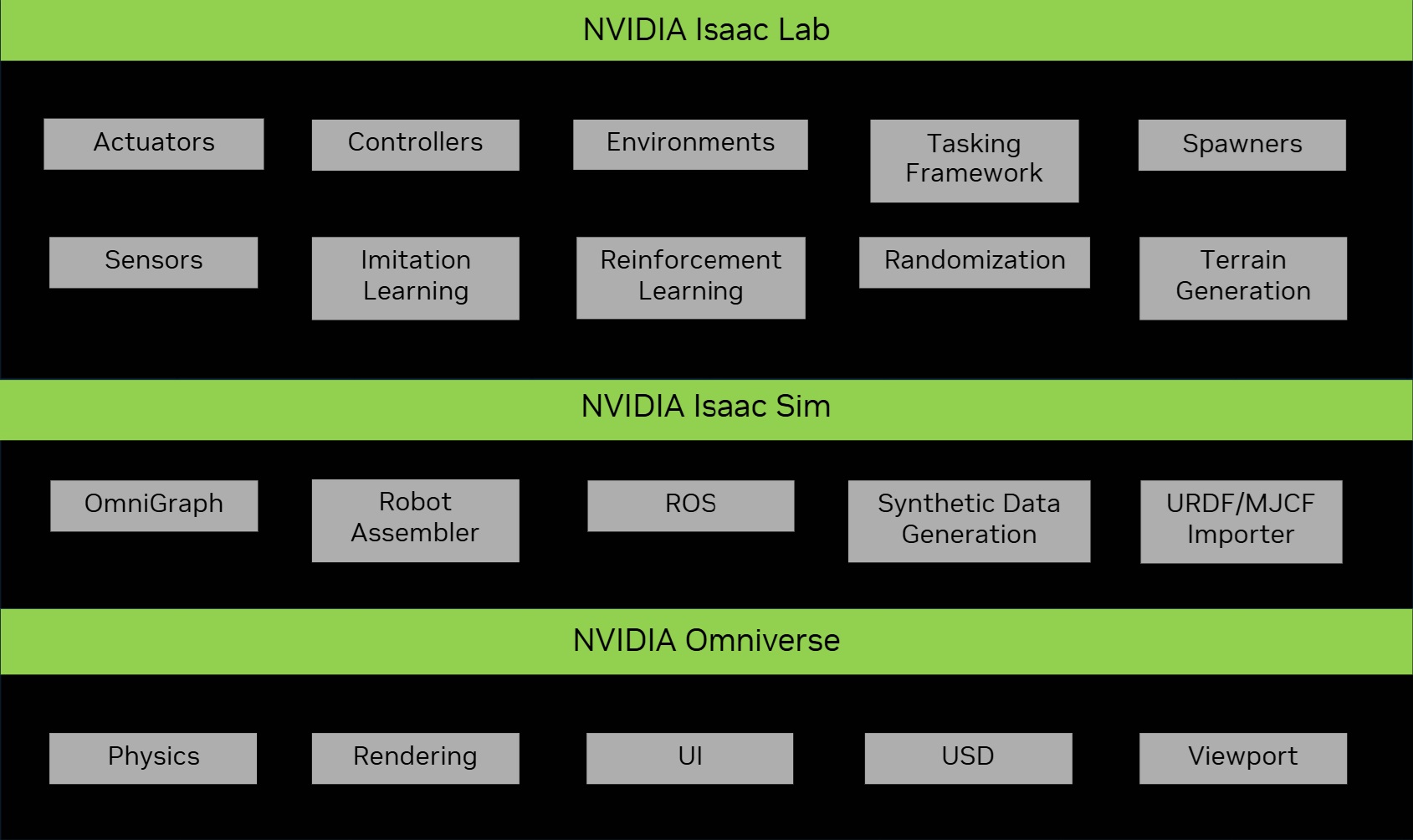
<p>Okay, so Nvidia Isaac Sim and Isaac Lab are both part of this ecosystem called “Omniverse”, which honestly can be pretty confusing at first.</p>

<p><img src="/assets/images/posts/double-pendulum/isaac_env.jpg" alt="Isaac Env" class="img-large" />
<em>Source: <a href="https://isaac-sim.github.io/IsaacLab/main/source/setup/ecosystem.html">Isaac Lab Documentation</a></em></p>

<p>Think of Omniverse as the “operating system” for 3D simulation. Isaac Sim sits on top of that and focuses on robotics simulation. It works with ROS, URDF, and all those other robotics standards. Then Isaac Lab sits on top of Isaac Sim and lets you do reinforcement learning with your robots.</p>

<p>Beyond Omniverse, Nvidia also has:</p>
<ul>
  <li><strong>Nvidia Cosmos</strong>: For generating realistic synthetic 3D worlds and videos</li>
  <li><strong>Nvidia Gr00t</strong>: A general purpose foundation model to control humanoid robots</li>
  <li><strong>Isaac ROS</strong>: A collection of ROS packages built to be accelerated on Nvidia GPUs</li>
</ul>

<p>In our case, we’ll build our robot within Isaac Sim and train it using reinforcement learning with Isaac Lab.</p>

<h2 id="lets-build-our-pendulum">Let’s build our pendulum</h2>

<p>I designed the double pendulum in Onshape. I have more experience with SolidWorks, but Onshape was easy to pick up. Everything is in the cloud, it has a built-in versioning system, and it’s straightforward to export to URDF format.</p>

<p><strong>What is URDF?</strong> URDF (Unified Robot Description Format) is basically an XML file that describes your robot. Things like its parts, joints, what it looks like, and how it collides with stuff. It’s the standard way to describe robots in ROS and most simulation tools, including Isaac Sim. We need it because Isaac Sim reads these files to figure out how to load and simulate our robot.</p>

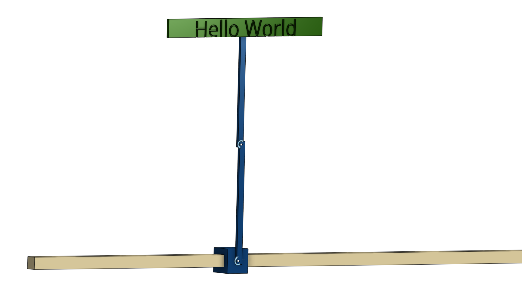
<p>As if balancing an inverted double pendulum wasn’t hard enough, I decided to add a small sign to the second arm to throw it off balance even more.</p>

<p>The double pendulum consists of:</p>
<ul>
  <li>A rail (fixed base)</li>
  <li>A cart that slides along the rail (controlled by the agent)</li>
  <li>A first arm attached to the cart</li>
  <li>A second arm attached to the first arm</li>
  <li>A small sign attached to the second arm</li>
</ul>

<p><img src="/assets/images/posts/double-pendulum/onshape.png" alt="Onshape" class="img-large" /></p>

<p>The tricky part? The agent can only control the horizontal force on the cart. It has to figure out how to keep both pendulum arms standing upright.</p>

<h2 id="manually-balancing-our-pendulum">Manually balancing our pendulum</h2>

<p>After importing the URDF into Isaac Sim, I made sure everything worked. I spent a while tweaking the joint physics, things like stiffness and damping for the cart sliding on the rail, to make it behave as realistically as possible. This matters a lot because if your simulation physics are realistic, your robot will work better when you try it on real hardware. That’s a whole topic on its own, so I’ll save the details for another time.</p>

<p>I tried to balance the pendulum manually using the cart controls. Let me tell you, it’s incredibly hard! The double pendulum is a chaotic system, and even small errors compound quickly. But we live in 2025 now, and we have AI to do the tedious work for us, even balance our pendulums.</p>

<video class="img-large" autoplay="" loop="" muted="" playsinline="">
  <source src="/assets/images/posts/double-pendulum/manual_trial.mp4" type="video/mp4" />
</video>

<h2 id="its-training-time">It’s training time</h2>

<p>I created a new project in Isaac Lab using their template system. Everything, loading the URDF, setting up joints, configuring physics, it’s all done through code.</p>

<p>You can find the code on Github <a class="link-prominent" href="https://github.com/NRdrgz/DoublePendulumIsaacLab" target="_blank" rel="noopener">here</a>
.</p>

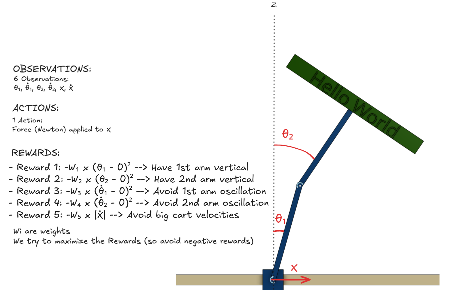
<p>Now here’s the key part of reinforcement learning: we need to define rewards. The model trains a bunch of instances at the same time (4,096 in my case!) and tries to get the highest total reward.</p>

<p>For our inverted double pendulum, we want both arms to stay straight up. Here’s the basic reward setup:</p>

<ol>
  <li>
    <p><strong>Upright position reward</strong>: We penalize the agent when the arms tilt away from vertical. The more they tilt, the bigger the penalty. This is the main goal.</p>
  </li>
  <li>
    <p><strong>Smooth motion rewards</strong>: We also penalize high speeds, both how fast the arms swing and how fast the cart moves. This stops the robot from being all jerky and wobbly, and makes it move smoothly instead.</p>
  </li>
</ol>

<p>Each reward has a weight that says how important it is. The agent gets these rewards every step of the simulation. The neural network figures out how to balance all these competing goals by trying different things across thousands of parallel simulations.</p>

<p><img src="/assets/images/posts/double-pendulum/rewards.png" alt="Rewards" class="img-large" /></p>

<p>With this reward setup, we’re ready to train! I used the PPO (Proximal Policy Optimization) algorithm with the skrl library, which works really well for this kind of continuous control task.</p>

<p>Finding the right weights for these rewards was one of the biggest headaches. If the upright position reward is too weak, the agent just never learns to balance. If the smooth motion penalties are too strong, the agent gets too cautious and can’t make quick corrections when things go wrong. I spent a lot of time tweaking these weights, running training, watching what happened, and adjusting.</p>

<p>There are a few ways to make this easier. One common trick is curriculum learning. Start with simpler goals (like just balancing from an upright position) and slowly add more complex rewards. Another option is to use reward normalization or scaling, which automatically balances the different reward parts. Some people also use automated tools to search for the best hyperparameters. For this project, I did it the manual way, but those techniques can save you a ton of time.</p>

<p>Here is a gif showing our 4,096 instances learning how to balance themselves in parallel.</p>

<video class="img-large" autoplay="" loop="" muted="" playsinline="">
  <source src="/assets/images/posts/double-pendulum/training.mp4" type="video/mp4" />
</video>

<h2 id="under-the-hood">Under the hood</h2>

<p>If you want to understand the magic behind the scenes, check out <a class="link-prominent" href="https://nrdrgz.github.io/2025/12/02/double-pendulum-rl-deep-dive/" target="_blank" rel="noopener">Part 2: Behind the scenes</a>
. I explain how reinforcement learning actually works, what PPO does, and how neural networks learn from rewards.</p>

<p>For now, just know that the agent tries different things, figures out what works, and gets better over millions of simulation steps.</p>

<h2 id="our-trained-policy">Our trained policy</h2>

<p>After just 20 minutes of training (on my 4080 Super), we have a policy that “learned” how to swing up the arms and keep them balanced. Check out this gif where I push the robot around to mess it up, and it recovers back to standing upright.</p>

<video class="img-large" autoplay="" loop="" muted="" playsinline="">
  <source src="/assets/images/posts/double-pendulum/trained.mp4" type="video/mp4" />
</video>

<div class="callout">
This shows how powerful reinforcement learning can be. You could use a traditional PID controller to balance the pendulum, but the RL model also figured out how to swing it up from rest. And it did all of this without any labeled training data. The agent learned purely through trial and error in simulation.
</div>

<h2 id="whats-next">What’s next?</h2>

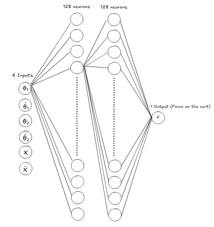
<p>So now we have a trained neural network! It takes in the positions and speeds of both arms, plus the position and speed of the cart, and spits out a force to apply to the cart to keep everything balanced.</p>

<p>The neural network itself is pretty simple. It’s just a feedforward network. You give it the current state, it goes through a few hidden layers, and out comes the force. The “magic” is all in the weights, which were learned through millions of trials in simulation.</p>

<p><img src="/assets/images/posts/double-pendulum/neural_net.png" alt="NN" class="img-medium" />
<em>Note: All neurons in each layer are interconnected to neurons in adjacent layers.</em></p>

<p>The next big step would be to take this neural network and put it on a real robot with real motors. This is called “sim to real” transfer, and that’s where things get really interesting. Having realistic physics in your simulation becomes super important here. You need to make sure your joint stiffness, controller force, and frequency are actually possible in the real world.</p>

<p>For example, in our simulation, we set up a force of up to 100N and a 60Hz control frequency.
This means our real-time controller needs to:</p>
<ul>
  <li>Read sensors</li>
  <li>Run the neural network (do inference)</li>
  <li>Send commands to the motor</li>
</ul>

<p>All in just 16.67ms (one control cycle).</p>

<h2 id="how-to-walk-from-there">How to walk from there?</h2>

<p>We’ve trained a system with 3 degrees of freedom (the cart position and two arm angles). A humanoid robot has something like 20 to 30 degrees of freedom just for walking. The idea is the same. Define rewards, train in simulation, and transfer to reality. But the complexity and computing power needed goes way up.</p>

<div class="callout">
Reinforcement learning is just one of many cool techniques in modern robotics, its big advantage being that you do not need training data, but you do need to build a simulation of your robot. I'll write more articles about imitation learning, vision language action (VLA) models, and other exciting stuff happening in the field!
</div>]]></content><author><name>Nicolas Rodriguez</name></author><summary type="html"><![CDATA[Learn how to use Isaac Lab to train an inverted double pendulum to stay upright]]></summary></entry><entry><title type="html">(Part 2) … and used Foxglove through the journey</title><link href="https://nrdrgz.github.io/2025/10/22/foxglove-studio-robotics-visualization/" rel="alternate" type="text/html" title="(Part 2) … and used Foxglove through the journey" /><published>2025-10-22T00:00:00+00:00</published><updated>2025-10-22T00:00:00+00:00</updated><id>https://nrdrgz.github.io/2025/10/22/foxglove-studio-robotics-visualization</id><content type="html" xml:base="https://nrdrgz.github.io/2025/10/22/foxglove-studio-robotics-visualization/"><![CDATA[<p>This article is a continuation of the previous one <a class="link-prominent" href="https://nrdrgz.github.io/2025/10/21/building-just1-autonomous-robot/" target="_blank" rel="noopener">Just1: How I built a small autonomous robot …</a>
. <br />
<em>I am in no way affiliated with Foxglove, and this article only reflects my personal experience.</em></p>
<div class="story-bar">
Coming from a company where dozens of engineers work on a single tool to visualize sensor data, I knew I couldn't afford the time and resources to reinvent the wheel for my personal robotics projects. That's when I discovered Foxglove, and it completely changed how I approach robotics development.
</div>

<h2 id="the-problem-visualizing-robot-data">The Problem: Visualizing Robot Data</h2>

<p>When building autonomous robots, you’re dealing with a constant stream of data from multiple sensors: lidar scans, camera feeds, IMU readings, motor commands, and navigation states. The challenge isn’t just collecting this data. It’s making sense of it all in real-time.</p>

<p>You can easily spend more time debugging visualization tools than actually working on your robot’s algorithms.</p>

<p>Traditional approaches to visualize your data in robotics usually include:</p>
<ul>
  <li><strong>Command-line tools</strong>: Functional but not intuitive for complex data</li>
  <li><strong>Custom web interfaces</strong>: Time-consuming to build and maintain</li>
  <li><strong>Python/Jupyter</strong>: Flexible and fast to iterate, but mostly offline and manual</li>
  <li><strong>ROS2 built-in tools (Rviz)</strong>: Powerful but with a steep learning curve and ugly UI</li>
</ul>

<h2 id="enter-foxglove">Enter Foxglove</h2>

<p>Foxglove is a powerful robotics visualization tool that works seamlessly with ROS2. It’s like having a professional-grade cockpit for your robot, but without the months of development time.</p>

<h3 id="what-makes-foxglove-special">What Makes Foxglove Special</h3>

<p><strong>Real-time Data Visualization</strong>: Foxglove connects directly to your robot’s ROS2 topics and displays sensor data in real-time. Whether it’s lidar point clouds, camera feeds, or navigation paths, everything updates live as your robot operates.</p>

<p><strong>Multi-Panel Interface</strong>: Unlike single-purpose tools, Foxglove lets you create custom dashboards with multiple panels. You can have a 3D map, camera feed, sensor graphs, and control panels all in one view.</p>

<p><strong>No Coding Required</strong>: The interface is drag-and-drop. You add panels, configure them, and start visualizing immediately. No need to write custom visualization code.</p>

<p><strong>Recording and Playback</strong>: You can record all your robot’s data and replay it later for analysis. This is invaluable for debugging issues that happened hours ago.</p>

<h2 id="how-i-used-foxglove-with-just1">How I Used Foxglove with Just1</h2>

<p>For my Just1 robot project, Foxglove became the central hub for development and testing. Here’s how I used it:</p>

<h3 id="1-real-time-monitoring">1. Real-Time Monitoring</h3>
<ul>
  <li><strong>3D Map Panel</strong>: Visualizes the robot’s SLAM map and current position</li>
  <li><strong>Camera Panel</strong>: Shows the camera feed for visual feedback</li>
  <li><strong>Plot Panel</strong>: Displays sensor data like IMU readings and motor speeds</li>
</ul>

<h3 id="2-navigation-control">2. Navigation Control</h3>
<ul>
  <li><strong>2D Pose Panel</strong>: Click on the map to send navigation goals</li>
  <li><strong>Path Visualization</strong>: See the planned path and current trajectory</li>
  <li><strong>Obstacle Detection</strong>: Monitor lidar data for obstacle avoidance</li>
</ul>

<p><img src="/assets/images/posts/foxglove/3d.jpg" alt="Navigation Control" class="img-large" /></p>

<h3 id="3-debugging-and-analysis">3. Debugging and Analysis</h3>
<ul>
  <li><strong>Topic Monitor</strong>: Track all ROS2 topics and their message rates</li>
  <li><strong>Log Analysis</strong>: Review recorded data to understand what went wrong</li>
</ul>

<p><img src="/assets/images/posts/foxglove/debug.jpg" alt="Debugging" class="img-large" /></p>

<h2 id="how-i-installed-it">How I installed it</h2>

<p>There are many ways to connect Foxglove to your robot depending on your stack. In my case, since I was using ROS2, it was as simple as adding another node. I followed their documentation <a class="link-prominent" href="https://docs.foxglove.dev/docs/getting-started/frameworks/ros2" target="_blank" rel="noopener">here</a>
.<br />
Check out my code <a class="link-prominent" href="https://github.com/NRdrgz/Just1/blob/main/Bot/Software/src/just1_bringup/launch/just1.launch.py#L167" target="_blank" rel="noopener">here</a>
 where I add the foxglove-bridge node.<br />
You can whitelist a list of topics and data will start flowing into your Foxglove app.<br />
Want to add a Camera Panel? Just send over your <code class="language-plaintext highlighter-rouge">/camera/video</code> topic.</p>

<p>Installing the UI on your computer is even easier. Just <a class="link-prominent" href="https://foxglove.dev/download" target="_blank" rel="noopener">download Foxglove</a>
 and follow the steps <a class="link-prominent" href="https://docs.foxglove.dev/docs/getting-started/frameworks/ros2" target="_blank" rel="noopener">here again</a>
.</p>

<p><img src="/assets/images/posts/foxglove/connection.jpg" alt="Foxglove Connection" class="img-medium" /></p>

<h2 id="see-foxglove-in-action-with-my-just1-demo">See Foxglove in Action with My Just1 Demo</h2>

<p><a href="https://www.youtube.com/watch?v=m_tZ3eg-KsA" target="_blank">
  <img src="/assets/images/posts/just1/demo.png" alt="Watch the demo" style="width:1000px;" />
</a></p>

<h2 id="the-takeaway">The Takeaway</h2>

<p>Foxglove Studio transformed my robotics development from a frustrating, guesswork-heavy process into an intuitive, visual experience. It’s not just a tool. It’s a paradigm shift in how we interact with robot data.</p>

<p>The features I explored through the Just1 project only seem like the tip of the iceberg of what Foxglove can do, and I’m looking forward to experimenting more with it in future projects.</p>

<p><img src="/assets/images/posts/foxglove/iceberg.png" alt="FOxglove iceberg" class="img-medium" /></p>

<div class="callout">
Foxglove is really an awesome tool, and if you are looking to integrate it into your small hobbyist project or your huge company, check out their <a class="link-prominent" href="https://docs.foxglove.dev/docs" target="_blank" rel="noopener">official documentation</a>
 or <a class="link-prominent" href="https://foxglove.dev/blog?topic=all" target="_blank" rel="noopener">blog</a>
.
</div>]]></content><author><name>Nicolas Rodriguez</name></author><summary type="html"><![CDATA[How Foxglove Studio transformed my robotics development workflow and why it's become an essential tool for visualizing data and debugging]]></summary></entry><entry><title type="html">(Part 1) Just1: How I built a small autonomous robot …</title><link href="https://nrdrgz.github.io/2025/10/21/building-just1-autonomous-robot/" rel="alternate" type="text/html" title="(Part 1) Just1: How I built a small autonomous robot …" /><published>2025-10-21T00:00:00+00:00</published><updated>2025-10-21T00:00:00+00:00</updated><id>https://nrdrgz.github.io/2025/10/21/building-just1-autonomous-robot</id><content type="html" xml:base="https://nrdrgz.github.io/2025/10/21/building-just1-autonomous-robot/"><![CDATA[<p>Picture this: You’re sitting in your room, scrolling through robotics videos on YouTube, watching these incredible autonomous robots navigate through complex environments. The price tags? Thousands of dollars. The complexity? Intimidating. But what if I told you that you could build your own autonomous robot for just $250?</p>

<h2 id="the-genesis-of-an-idea">The Genesis of an Idea</h2>

<div class="story-bar">
It all started when I was working for an autonomous driving company in San Francisco. I was surrounded by tremendously smart people working on a very complex system. I already knew about robotics, mainly from the software and data side, but I wanted to better understand several other aspects: middleware, perception, planning, control, and more. Convinced that hands-on projects are the best way to learn and make progress, I started working on Just1. I wanted to build a small, affordable robot that could navigate manually or autonomously and avoid obstacles.
</div>

<p><img src="/assets/images/posts/just1/cartoon1.png" alt="Just1 Cartoon" class="img-medium" /></p>

<h2 id="the-hardware-challenge">The Hardware Challenge</h2>

<p>Building a robot on a budget means making some tough choices. Every component had to justify its cost, and every feature had to serve a clear purpose.</p>

<p><strong>The Brain</strong>: Raspberry Pi 4 (8GB) at $80 was my biggest expense, but it needed to handle real-time sensor processing, SLAM algorithms, and navigation planning. The Pi 5 would have been nice, but finding a reliable 5A power supply proved challenging. Looking back, the RAM isn’t much of a bottleneck since we’re using LIDAR instead of camera-only navigation. We’re much more constrained by CPU usage.</p>

<p><strong>The Eyes</strong>: This is where things got interesting. I originally planned to use only a camera for Visual SLAM (VSLAM), but after weeks of debugging and optimization, I ended up buying the cheapest 2D Lidar I could find. The LD19 Lidar at $70 became the cornerstone of the robot’s perception system.</p>

<p><strong>The Movement</strong>: Mecanum wheels were fun to work with. I initially wanted to experiment with them because they provide interesting control capabilities. These omnidirectional wheels allow the robot to move forward, backward, sideways, and rotate in place, making them perfect for tight spaces and precise positioning. Four TT motors with L298N drivers were the cheapest solution to control them.</p>

<p><strong>The Senses</strong>: An MPU6050 IMU ($3!) provides orientation data, while the optional Camera Module 3 adds visual feedback for future enhancements.</p>

<div class="story-bar">
The total cost breakdown: $250 for a fully functional autonomous robot. <br />
That's less than many people spend on a single component for their robotics projects!
</div>

<h2 id="the-software-stack-where-the-magic-happens">The Software Stack: Where the Magic Happens</h2>

<p>Hardware is just the beginning. The real challenge was making all these components work together seamlessly. I chose ROS2 as the middleware because it’s the industry standard for robotics, and learning it would be valuable for future projects. My main goal for this project was actually to get hands-on experience with ROS2 to better understand how it works.</p>

<p><strong>Navigation Stack</strong>: RTAB-Map handles SLAM (Simultaneous Localization and Mapping), creating a map of the environment while tracking the robot’s position. Nav2 provides the path planning and obstacle avoidance capabilities.</p>

<p><strong>Sensor Fusion</strong>: A Madgwick filter combines IMU data with other sensors for accurate orientation estimation.</p>

<p><strong>Visualization</strong>: Coming from a company where dozens of engineers work on a single tool to visualize sensor data, I couldn’t afford the time and resources to reinvent the wheel.
Foxglove Studio became my best friend during development. This powerful tool lets me visualize sensor data, monitor the robot’s state, and even send navigation goals through an intuitive interface.</p>

<h2 id="the-development-journey">The Development Journey</h2>

<p>Building Just1 wasn’t just about assembling hardware and writing code. It was a crash course in robotics engineering. Here are some of the key lessons I learned:</p>

<h3 id="lesson-1-start-simple-then-optimize">Lesson 1: Start Simple, Then Optimize</h3>
<p>My first version used JPEG encoding for the camera feed, which consumed massive CPU resources. Switching to H.264 encoding dramatically improved performance, but I didn’t need to spend time on that until late in the development. Sometimes the simplest solution isn’t the most efficient, but don’t spend time on issues you don’t have yet.</p>

<h3 id="lesson-2-documentation-is-everything">Lesson 2: Documentation is Everything</h3>
<p>Every wiring connection, every software configuration, every troubleshooting step. I documented it all. This wasn’t just for others who might want to build their own Just1, but for future me who would inevitably forget how I solved that one tricky bug at 2 AM.</p>

<h3 id="lesson-3-real-world-testing-reveals-everything">Lesson 3: Real-World Testing Reveals Everything</h3>
<p>Simulation is great, but there’s no substitute for real-world testing. Coming from the software world into hardware, you have to expect the unexpected. Your robot can fail or behave strangely simply because it’s out of battery. Light and shadows can play tricks on your sensor inputs.</p>

<p><a href="https://www.youtube.com/watch?v=m_tZ3eg-KsA" target="_blank">
  <img src="/assets/images/posts/just1/demo.png" alt="Watch the demo" style="width:1000px;" />
</a></p>

<h2 id="the-foxglove-revelation">The Foxglove Revelation</h2>

<p>One of the most surprising discoveries was how much Foxglove Studio transformed the development experience. This visualization tool became essential for:</p>

<ul>
  <li><strong>Real-time monitoring</strong>: Watching sensor data streams, camera feeds, and navigation status</li>
  <li><strong>Debugging</strong>: Visualizing the robot’s understanding of its environment</li>
  <li><strong>Control</strong>: Sending navigation goals through an intuitive interface</li>
  <li><strong>Analysis</strong>: Reviewing recorded data to understand what went wrong (or right)</li>
</ul>

<p>Foxglove turned what could have been a command-line nightmare into an intuitive, visual experience. It’s like having a cockpit for your robot. I’ve written a  <a class="link-prominent" href="https://nrdrgz.github.io/2025/10/22/foxglove-studio-robotics-visualization/" target="_blank" rel="noopener">dedicated blog post on Foxglove</a>
.</p>

<h2 id="the-bigger-picture">The Bigger Picture</h2>

<p>Building Just1 taught me that autonomous robotics doesn’t have to be prohibitively expensive or impossibly complex. Having previously worked with the famous <a class="link-prominent" href="https://github.com/TheRobotStudio/SO-ARM100" target="_blank" rel="noopener">SO-101</a>
, I’m proud to have built something similar for a small autonomous robot, complete with ROS2 integration.</p>

<p>The project is fully open-source, with complete documentation, CAD files, and software available for anyone who wants to build their own. I built Just1 mainly for myself, but I was proud to share it online and received great feedback. Just1 has been shared <a class="link-prominent" href="https://www.reddit.com/r/robotics/comments/1noj43w/meet_just1_a_small_mecanumwheel_autonomous_robot/" target="_blank" rel="noopener">on Reddit</a>
 and appeared in the <a class="link-prominent" href="https://www.weeklyrobotics.com/weekly-robotics-330" target="_blank" rel="noopener">Weekly Robotics newsletter</a>
! I ended up meeting new people and having drinks with others who wanted to build their own Just1 and learn robotics. That’s the beauty of hardware!</p>

<h2 id="the-takeaway">The Takeaway</h2>

<p>The best way to learn about something is just to dive into it and build a project out of it. In the software world, it’s very easy to do. You just need a computer and you can start coding. But with Just1, I realized that the same is also possible in hardware. You can build a very simple robot and learn principles that are applied in robotaxis roaming the streets of San Francisco.</p>

<p>The journey from idea to working robot was filled with challenges, late-night debugging sessions, and moments of pure joy when everything finally clicked. But most importantly, it showed me that the barrier to entry in robotics isn’t as high as it might seem.</p>

<p>So, what’s your “Just1” project? What have you been wanting to build but thought was too complex or expensive? Sometimes, the best way to find out is to just start building.</p>

<div class="callout">
Want to build your own Just1? Check out the complete project documentation, CAD files, and software at the <a class="link-prominent" href="https://github.com/NRdrgz/Just1" target="_blank" rel="noopener">Just1 GitHub repository</a>
. All the code, schematics, and build instructions are freely available for anyone who wants to dive into autonomous robotics.
</div>]]></content><author><name>Nicolas Rodriguez</name></author><summary type="html"><![CDATA[How I built Just1, a $250 Mecanum wheel robot that can navigate and avoid obstacles autonomously.]]></summary></entry><entry><title type="html">Catch ‘Em All: Unlocking the Secrets of the Coupon Collector’s Problem</title><link href="https://nrdrgz.github.io/2025/10/01/coupon-collectors-problem/" rel="alternate" type="text/html" title="Catch ‘Em All: Unlocking the Secrets of the Coupon Collector’s Problem" /><published>2025-10-01T00:00:00+00:00</published><updated>2025-10-01T00:00:00+00:00</updated><id>https://nrdrgz.github.io/2025/10/01/coupon-collectors-problem</id><content type="html" xml:base="https://nrdrgz.github.io/2025/10/01/coupon-collectors-problem/"><![CDATA[<div class="story-bar">
The idea for this article started when I was at work with some friends.  <br />
One of them had just bought "Panini" cards. If you don't know about them, they are collectible cards, mainly revolving around football. <br />
<br />
My friend had bought 100 cards and was complaining that with his bad luck, he would surely end up with many duplicates. Being the geeks that we are, we jumped to the whiteboard and started to predict how many duplicates he would draw. <br />
<br />
The problem turned out to be a bit more complex than we originally anticipated!
</div>

<p>This problem is called the Coupon Collector’s Problem!</p>

<p><img src="/assets/images/posts/coupon-collector/1.jpg" alt="Coupon Collector's Problem Illustration" class="img-medium" /></p>

<h2 id="simple-approach-to-the-problem">Simple approach to the problem</h2>

<p>To simplify the approach to the problem, let’s say that we are collecting monsters, and we are getting these monsters from “surprise boxes”. For now we’ll assume that there are 100 different monsters with the same probability of getting all of them.</p>

<p>It is your first opening of a box.
The probability of getting a new monster is … well 1, as you have no other monsters.
For your second opening of a box, the probability of getting a new different one is \(\frac{99}{100}\). Indeed, there is a slight “chance” (or bad luck) of \(\frac{1}{100}\) that you’ll get the same monster as your first opening.</p>

<p>To generalize our finding, if we already have \(k\) different monsters, the probability of getting a new monster out of a pool of \(N\) monsters (in our case \(N = 100\)) is:</p>

\[P(\text{new monster}) = \frac{N-k}{N}\]

<ul>
  <li>If we already have 99 monsters, the probability of finding a new one (the ultimate one!) is \(\frac{1}{100}\)</li>
</ul>

<p>This follows a geometric distribution with parameter \(\frac{N-k}{N}\).
The expectation of this geometric distribution is \(\frac{N}{N-k}\).
We can interpret this expectation as:</p>

<p>After already having \(k\) different monsters, we’d need to open on average \(\frac{N}{N-k}\) boxes to get a new one.</p>

<ul>
  <li>So if we already have 99 monsters, we’d need on average to open 100 boxes to have a new one.</li>
</ul>

<p>Let’s use this expectation formula.
If we have 0 monsters, the number of box openings to get a new one is:</p>

\[\frac{100}{100-0} = 1\]

<p>Once we have 1 monster, the number of box openings on average to get a new one is:</p>

\[\frac{100}{100-1} \approx 1.01\]

<p>Summing both, the average number of box openings to get 2 monsters is 2.01. As we’ve seen before, there is a slight chance that we’ll get the same monster after the 2 box openings.</p>

<p>Generalizing, in order to get \(k\) different monsters, we’ll need to open this amount of boxes:</p>

\[\frac{100}{100-0} + \frac{100}{100-1} + \frac{100}{100-2} + \dots + \frac{100}{100-(k-1)}\]

<p>Which we can also write:</p>

\[\sum_{i=1}^{k} \frac{100}{100-(i-1)}\]

<p>Let’s compute this sum in Python.</p>

<details>
<summary><strong>Show code</strong></summary>


<figure class="highlight"><pre><code class="language-python" data-lang="python"><span class="kn">import</span> <span class="nn">numpy</span> <span class="k">as</span> <span class="n">np</span>
<span class="kn">import</span> <span class="nn">matplotlib.pyplot</span> <span class="k">as</span> <span class="n">plt</span>
<span class="c1">#We can build the sum with a for loop
</span>
<span class="n">N</span> <span class="o">=</span> <span class="mi">100</span>

<span class="k">def</span> <span class="nf">openbox_depending_on_monster</span><span class="p">(</span><span class="n">k</span><span class="p">):</span>
    <span class="n">total</span> <span class="o">=</span> <span class="mi">0</span>
    <span class="k">for</span> <span class="n">i</span> <span class="ow">in</span> <span class="nb">range</span><span class="p">(</span><span class="mi">1</span><span class="p">,</span> <span class="n">k</span> <span class="o">+</span> <span class="mi">1</span><span class="p">):</span>
        <span class="n">total</span> <span class="o">+=</span> <span class="n">N</span> <span class="o">/</span> <span class="p">(</span><span class="n">N</span> <span class="o">-</span> <span class="p">(</span><span class="n">i</span> <span class="o">-</span> <span class="mi">1</span><span class="p">))</span>
    <span class="k">return</span> <span class="n">total</span>

<span class="c1">#or with a vectorized approach
</span>
<span class="k">def</span> <span class="nf">openbox_depending_on_monster_np</span><span class="p">(</span><span class="n">k</span><span class="p">):</span>
    <span class="c1"># np.arange creates an array starting from 1 up to k
</span>    <span class="n">indices</span> <span class="o">=</span> <span class="n">np</span><span class="p">.</span><span class="n">arange</span><span class="p">(</span><span class="mi">1</span><span class="p">,</span> <span class="n">k</span> <span class="o">+</span> <span class="mi">1</span><span class="p">)</span>
    <span class="c1"># Directly compute the terms using vectorized operations and compute the sum
</span>    <span class="n">total</span> <span class="o">=</span> <span class="n">np</span><span class="p">.</span><span class="nb">sum</span><span class="p">(</span><span class="n">N</span> <span class="o">/</span> <span class="p">(</span><span class="n">N</span> <span class="o">-</span> <span class="p">(</span><span class="n">indices</span> <span class="o">-</span> <span class="mi">1</span><span class="p">)))</span>
    <span class="k">return</span> <span class="n">total</span>

<span class="k">print</span><span class="p">(</span><span class="s">"So to get 95% of the monsters (95) we'd need to open {} boxes"</span><span class="p">.</span><span class="nb">format</span><span class="p">(</span><span class="nb">int</span><span class="p">(</span><span class="n">openbox_depending_on_monster_np</span><span class="p">(</span><span class="mi">95</span><span class="p">))))</span>
<span class="k">print</span><span class="p">(</span><span class="s">"And to be sure to have all 100 distinct monsters we'd need to open on average {} boxes"</span><span class="p">.</span><span class="nb">format</span><span class="p">(</span><span class="nb">int</span><span class="p">(</span><span class="n">openbox_depending_on_monster_np</span><span class="p">(</span><span class="mi">100</span><span class="p">))))</span></code></pre></figure>


</details>

<div class="callout">
To get 95 distinct monsters out of our 100 available monsters, we'd have to open 290 boxes, and in order to get all the 100 monsters, we'd have to open 518 boxes!
</div>

<p>We can also plot the evolution of the number of distinct monsters, depending on the number of box openings:</p>

<p><img src="/assets/images/posts/coupon-collector/6.jpg" alt="Monster collection chart" class="img-medium" /></p>

<details>
<summary><strong>Show code</strong></summary>


<figure class="highlight"><pre><code class="language-python" data-lang="python"><span class="c1"># Range of k values from 1 to 100
</span><span class="n">N</span> <span class="o">=</span> <span class="mi">100</span>
<span class="n">k_values</span> <span class="o">=</span> <span class="n">np</span><span class="p">.</span><span class="n">arange</span><span class="p">(</span><span class="mi">1</span><span class="p">,</span> <span class="n">N</span><span class="p">)</span>
<span class="c1"># Compute the sum for each k
</span><span class="n">sum_results</span> <span class="o">=</span> <span class="p">[</span><span class="n">openbox_depending_on_monster_np</span><span class="p">(</span><span class="n">k</span><span class="p">)</span> <span class="k">for</span> <span class="n">k</span> <span class="ow">in</span> <span class="n">k_values</span><span class="p">]</span>

<span class="c1"># Create the plot
</span><span class="n">plt</span><span class="p">.</span><span class="n">figure</span><span class="p">(</span><span class="n">figsize</span><span class="o">=</span><span class="p">(</span><span class="mi">10</span><span class="p">,</span> <span class="mi">6</span><span class="p">))</span>
<span class="n">plt</span><span class="p">.</span><span class="n">plot</span><span class="p">(</span><span class="n">sum_results</span><span class="p">,</span> <span class="n">k_values</span><span class="p">,</span> <span class="n">label</span><span class="o">=</span><span class="s">' '</span><span class="p">)</span>
<span class="n">plt</span><span class="p">.</span><span class="n">xlabel</span><span class="p">(</span><span class="s">'Number of box openings'</span><span class="p">)</span>
<span class="n">plt</span><span class="p">.</span><span class="n">ylabel</span><span class="p">(</span><span class="s">'Number of distinct monsters'</span><span class="p">)</span>
<span class="n">plt</span><span class="p">.</span><span class="n">title</span><span class="p">(</span><span class="s">'Number of distinct monsters depending on the number of box openings'</span><span class="p">)</span>
<span class="n">plt</span><span class="p">.</span><span class="n">grid</span><span class="p">(</span><span class="bp">True</span><span class="p">)</span>
<span class="n">plt</span><span class="p">.</span><span class="n">legend</span><span class="p">()</span>
<span class="n">plt</span><span class="p">.</span><span class="n">show</span><span class="p">()</span></code></pre></figure>


</details>

<p>We can see that the more monsters we get, the harder it is to find new ones!</p>

<h2 id="the-opposite-approach-to-the-problem--a-bit-more-complex">The opposite approach to the problem — a bit more complex</h2>

<p>What if we approach the problem from the other side?
How many distinct monsters do we get after opening \(k\) boxes?</p>

<p><img src="/assets/images/posts/coupon-collector/7.jpg" alt="Opposite approach visualization" class="img-medium" /></p>

<p>Well, we could always look at our charts above and deduce that, but from a statistical point of view, it would look like this:</p>

<p>The probability that monster \(i\) has not been picked after \(k\) attempts is:</p>

\[\left(\frac{99}{100}\right)^k\]

<p>So the probability that monster \(i\) has been picked at least once is:</p>

\[1 - \left(\frac{99}{100}\right)^k\]

<p>Given that each of the 100 monsters has the same probability of appearing, we can use the linearity of expectation to find the expected number of different monsters seen after \(k\) attempts:</p>

\[E(k) = 100 \left(1 - \left(\frac{99}{100}\right)^k\right)\]

<details>
<summary><strong>Show code</strong></summary>


<figure class="highlight"><pre><code class="language-python" data-lang="python"><span class="n">N</span> <span class="o">=</span> <span class="mi">100</span>

<span class="k">def</span> <span class="nf">monster_depending_on_openbox</span><span class="p">(</span><span class="n">k</span><span class="p">):</span>
    <span class="n">total</span> <span class="o">=</span> <span class="n">N</span><span class="o">*</span><span class="p">(</span><span class="mi">1</span><span class="o">-</span><span class="p">((</span><span class="n">N</span><span class="o">-</span><span class="mi">1</span><span class="p">)</span><span class="o">/</span><span class="n">N</span><span class="p">)</span><span class="o">**</span><span class="n">k</span><span class="p">)</span>
    <span class="k">return</span> <span class="n">total</span>

<span class="k">print</span><span class="p">(</span><span class="s">"So after opening 100 boxes, we'll have on average {} different monsters"</span><span class="p">.</span><span class="nb">format</span><span class="p">(</span><span class="nb">int</span><span class="p">(</span><span class="n">monster_depending_on_openbox</span><span class="p">(</span><span class="mi">100</span><span class="p">))))</span></code></pre></figure>


</details>

<div class="callout">
After opening 100 boxes, we'll have on average 63 different monsters!
</div>

<h2 id="non-uniform-distribution--even-more-complex">Non-uniform distribution — even more complex</h2>

<p>Now, what happens if the probabilities of obtaining each monster are not uniform when opening a box?
Let’s say we have 90 monsters with a probability of being found of \(\frac{1}{91}\) and 10 rare monsters with a probability of being found of \(\frac{1}{910}\).</p>

<p>How many box openings will it take to collect all 100 different monsters?</p>

<p>Well, the mathematical approach gets a bit more complicated, so we’ll venture into the world of simulation with Monte Carlo methods.</p>

<h3 id="monte-carlo-methods">Monte Carlo methods</h3>

<p>Monte Carlo methods are a type of computational algorithm used to solve problems through random sampling.
We are going to simulate multiple series of box openings until we reach our target of unique monsters, and then we will see on average how many box openings we needed.</p>

<p><img src="/assets/images/posts/coupon-collector/11.jpg" alt="Monte Carlo simulation" class="img-medium" /></p>

<details>
<summary><strong>Show code</strong></summary>


<figure class="highlight"><pre><code class="language-python" data-lang="python"><span class="kn">import</span> <span class="nn">numpy</span> <span class="k">as</span> <span class="n">np</span>

<span class="c1"># Define probabilities for each monster
</span><span class="n">probabilities</span> <span class="o">=</span> <span class="p">[</span><span class="mi">1</span><span class="o">/</span><span class="mi">91</span><span class="p">]</span> <span class="o">*</span> <span class="mi">90</span> <span class="o">+</span> <span class="p">[</span><span class="mi">1</span><span class="o">/</span><span class="mi">910</span><span class="p">]</span> <span class="o">*</span> <span class="mi">10</span>  
<span class="c1">#probabilities = [1/100] * 100 #we can do that if we want to simulate with uniform distribution
</span><span class="n">probabilities</span> <span class="o">=</span> <span class="n">np</span><span class="p">.</span><span class="n">array</span><span class="p">(</span><span class="n">probabilities</span><span class="p">)</span> <span class="o">/</span> <span class="nb">sum</span><span class="p">(</span><span class="n">probabilities</span><span class="p">)</span>  <span class="c1"># Normalize probabilities
</span>
<span class="c1"># Number of total monsters
</span><span class="n">total_monsters</span> <span class="o">=</span> <span class="nb">len</span><span class="p">(</span><span class="n">probabilities</span><span class="p">)</span>

<span class="c1"># Target number of unique monsters (we want to reach 100 of unique monsters)
</span><span class="n">target_unique_monsters</span> <span class="o">=</span> <span class="mi">100</span>

<span class="c1"># Function to simulate opening boxes until we reach the target
</span><span class="k">def</span> <span class="nf">simulate_boxes</span><span class="p">():</span>
    <span class="n">collected_monsters</span> <span class="o">=</span> <span class="nb">set</span><span class="p">()</span>
    <span class="n">box_count</span> <span class="o">=</span> <span class="mi">0</span>
    <span class="k">while</span> <span class="nb">len</span><span class="p">(</span><span class="n">collected_monsters</span><span class="p">)</span> <span class="o">&lt;</span> <span class="n">target_unique_monsters</span><span class="p">:</span>
        <span class="n">monster</span> <span class="o">=</span> <span class="n">np</span><span class="p">.</span><span class="n">random</span><span class="p">.</span><span class="n">choice</span><span class="p">(</span><span class="n">total_monsters</span><span class="p">,</span> <span class="n">p</span><span class="o">=</span><span class="n">probabilities</span><span class="p">)</span>
        <span class="n">collected_monsters</span><span class="p">.</span><span class="n">add</span><span class="p">(</span><span class="n">monster</span><span class="p">)</span>
        <span class="n">box_count</span> <span class="o">+=</span> <span class="mi">1</span>
    <span class="k">return</span> <span class="n">box_count</span>

<span class="c1"># Number of simulations
</span><span class="n">num_simulations</span> <span class="o">=</span> <span class="mi">10000</span>
<span class="n">results</span> <span class="o">=</span> <span class="p">[</span><span class="n">simulate_boxes</span><span class="p">()</span> <span class="k">for</span> <span class="n">_</span> <span class="ow">in</span> <span class="nb">range</span><span class="p">(</span><span class="n">num_simulations</span><span class="p">)]</span>

<span class="c1"># Calculate the average number of boxes needed
</span><span class="n">average_boxes</span> <span class="o">=</span> <span class="n">np</span><span class="p">.</span><span class="n">mean</span><span class="p">(</span><span class="n">results</span><span class="p">)</span>
<span class="k">print</span><span class="p">(</span><span class="s">"To have all 100 distinct monsters we'd need to open on average {} boxes"</span><span class="p">.</span><span class="nb">format</span><span class="p">(</span><span class="nb">int</span><span class="p">(</span><span class="n">average_boxes</span><span class="p">)))</span></code></pre></figure>


</details>

<div class="callout">
To have all 100 distinct monsters, we'd have to open on average 2658 boxes!
</div>

<p>We can see how this addition of rarer monsters drastically increases the number of boxes we have to open to collect them all!</p>

<p>This number is an average, but each round of the simulation got a different number of box openings to get all the monsters. We can even visualize the distribution of the number of openings needed in each round of the simulation.</p>

<details>
<summary><strong>Show code</strong></summary>


<figure class="highlight"><pre><code class="language-python" data-lang="python"><span class="kn">import</span> <span class="nn">matplotlib.pyplot</span> <span class="k">as</span> <span class="n">plt</span>

<span class="c1"># Plot the distribution of results from the simulations
</span><span class="n">plt</span><span class="p">.</span><span class="n">hist</span><span class="p">(</span><span class="n">results</span><span class="p">,</span> <span class="n">bins</span><span class="o">=</span><span class="mi">30</span><span class="p">,</span> <span class="n">color</span><span class="o">=</span><span class="s">'skyblue'</span><span class="p">,</span> <span class="n">edgecolor</span><span class="o">=</span><span class="s">'black'</span><span class="p">)</span>
<span class="n">plt</span><span class="p">.</span><span class="n">title</span><span class="p">(</span><span class="s">'Distribution of Boxes Needed to Collect all monsters'</span><span class="p">)</span>
<span class="n">plt</span><span class="p">.</span><span class="n">xlabel</span><span class="p">(</span><span class="s">'Number of Boxes'</span><span class="p">)</span>
<span class="n">plt</span><span class="p">.</span><span class="n">ylabel</span><span class="p">(</span><span class="s">'Frequency'</span><span class="p">)</span>
<span class="n">plt</span><span class="p">.</span><span class="n">grid</span><span class="p">(</span><span class="bp">True</span><span class="p">)</span>
<span class="n">plt</span><span class="p">.</span><span class="n">show</span><span class="p">()</span></code></pre></figure>


</details>

<p><img src="/assets/images/posts/coupon-collector/12.jpg" alt="Distribution chart" class="img-medium" /></p>

<h2 id="conclusion">Conclusion</h2>

<p>We’ve explored the Coupon Collector’s Problem from simple uniform distributions to complex scenarios with rare items. The math shows that collecting everything takes patience, especially when some items are much rarer than others.</p>

<p>Next time you open a pack or plan to collect something, remember: with math and persistence, even the most challenging collections can be completed!</p>

<p><img src="/assets/images/posts/coupon-collector/13.jpg" alt="Final visualization" class="img-medium" /></p>]]></content><author><name>Nicolas Rodriguez</name></author><summary type="html"><![CDATA[Explore the mathematics behind collecting trading cards. How many items do you need to complete your set?]]></summary></entry></feed>